Smart Lock Audio Recognition
Overview
This tutorial is a guide towards building a Smart Lock model that can be executed on a cortex-M4 microcontroller. The SensiML Analytics Toolkit is used to capture and annotate the audio data and build a model using the TensorFlow package that is deployed and tested on the edge device. Similar methodology can be used to develop similar audio classification algorithms, such as keyword spotting, industrial sound recognition, and smart home devices that are sound activated.
Smart Lock Demo
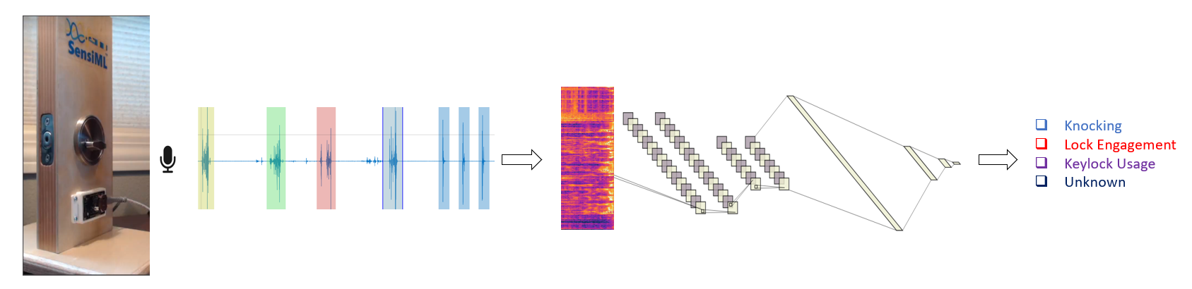
In most of these applications, the sound data is collected in the form of time series using a microphone mounted on an edge device that does the classification job by extracting and transforming the most significant features from the streaming data.
Note: In our example we will collect data at a sample rate of 16,000 samples per second (16 kHz). However, this tutorial is agnostic to the sample rate and all related parameters can be adjusted accordingly for other devices that function at different frequencies.
TIP: This tutorial is a more advanced audio use case. We will cover most of the basics of the SensiML Analytics Toolkit in this document, but to get a better understanding of the basics we recommend a more straightforward audio application such as Guitar Note Audio Recognition.
Objectives
This tutorial covers the following steps needed to build and deploy a smart lock model that is sensitive to several interesting audio events and is capable of confidently classifying them.
In this tutorial you will learn how to
Capture and label the audio data using the SensiML Data Studio software
Pre-process and stage the data using the SensiML Analytics Studio prior to building the model
Build the feature extraction pipelines with the SensiML Python SDK
Generate, train, and test a TensorFlow model using the SensiML Python SDK
Quantize and convert your TensorFlow model for compatibility with the 8-bit tiny devices
Test the model in the live data streaming mode in the Data Studio
Download and compile the model for the edge device of interest
Flash the model to the edge device and display the inferred classes in the SensiML Open Gateway user interface
What You Need to Get Started
This tutorial uses the SensiML Toolkit to handle collecting and annotating sensor data, creating a sensor preprocessing pipeline, and generating the firmware. Before you start, sign up for the free SensiML Community Edition to get access to the SensiML Analytics Toolkit.
Software
SensiML Data Studio (Windows 10) to record and label the audio data.
SensiML Analytics Studio for preparing data and managing pipelines and generating the appropriate Knowledge Pack to be deployed on the device of interest
Optional: SensiML Open Gateway or Putty/Tera Term to display the model outputs in real-time
Hardware
Select from our list of supported platforms
Use your own device by following the documentation for custom device firmware
We keep this tutorial agnostic to the chosen edge device. However, due to the complexity of the generated model, some devices might not have enough memory to store the model or generate the classifications in a reasonable time. Devices with the capability of accelerating the matrix arithmetic operations are recommended, but not necessary.
Door Lock
You can easily mount your sensor device next to a deadbolt mounted on a door, and generate each of your desired audio events - The simplest version of this demo can be recreated by only including one of the labels, say knocking. In this scenario, you can knock on a table and create a model using only the knocking event
Events of Interest (Audio Classes)
The main goal of this demo is to demonstrate how you can build a model that is aware of the ambient audio events around a door. The application may cover various activities including (but not limited to) lock picking, the usage of a wrong key, hammering the deadbolt, usage of a drilling tool to break into a room, knocking/pounding on the door, locking and unlocking a key, etc. Obviously, this is not an exhaustive list of all interesting events, and certainly many more classes can be included in this list.
Before covering all complex scenarios, and to better understand the basic concepts that need to be addressed in a fairly accurate model, we only choose a few simple audio events form the list to incorporate into our model.
These classes are
key-io: Inserting/Removing a key from the keyhole.
Locking/Unlocking: Turning the key inside the keyhole or using the knob
Knocking: Knocking on the door. In this demo we mainly focus on simple knocking with various intensities
Unknown: Anything else that is not one of the three previously defined labels. This is the output generated if the device is activated and triggered to return a classification by instances of intense background noise or other high intensity audio events that are not covered above.
Data Collection
1. Starting with the Data Studio
You will need to install the Data Studio in order to connect to the audio sensor and to collect data
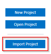
If you have already collected your sensor data, you can import them into the SensiML server following these steps.
If you are about to collect new data, please first consult with the Supported Devices section in the left menu bar of the SensiML documentation and flash the proper Data Collection Firmware to the device. If you don’t find your device in the list, please refer to this page to learn how to integrate your data into the Data Studio.
For the Silicon Labs xG24 Dev Kit, you can download the Data Collection Firmware for Microphone (16000 Hz) and flash it to the device following the steps described here.
Download the project
Import the project using the Data Studio
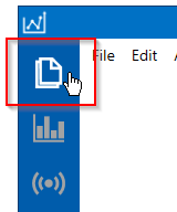
Click on the Project Explorer button in the top left navigation bar to view and open files in the project
You have the option to switch between different labeling sessions. In this example, each capture file is devoted to a particular event. We also set aside a set of shorter capture files for testing and validation purposes.
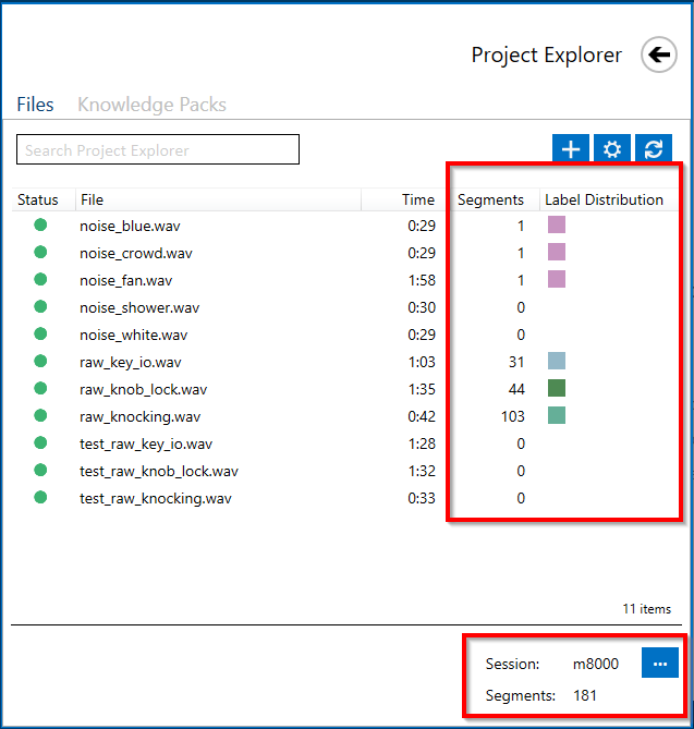
For clarity, we have generated two manual labeling sessions, i.e. m8000 and m8000_test, the former is used to annotate the files for the purpose of training, and the latter is dedicated for annotation of the test/validation files.
2. Recording Audio Data
Connecting to a Device
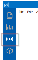
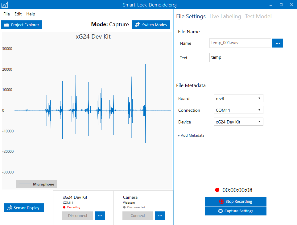
In the left navigation bar, click on the Live Capture button
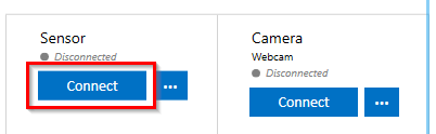
Click Connect to connect to your device
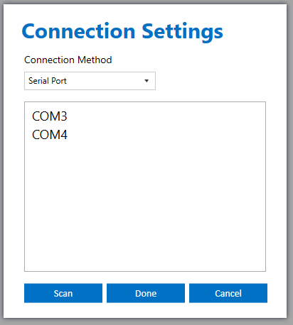
Click Scan to find the port number of your device.
Data Collection
You can set the max record time setting by clicking on the Capture Settings. We recommend for each set up similar events collect about 60 to 120 seconds of data.
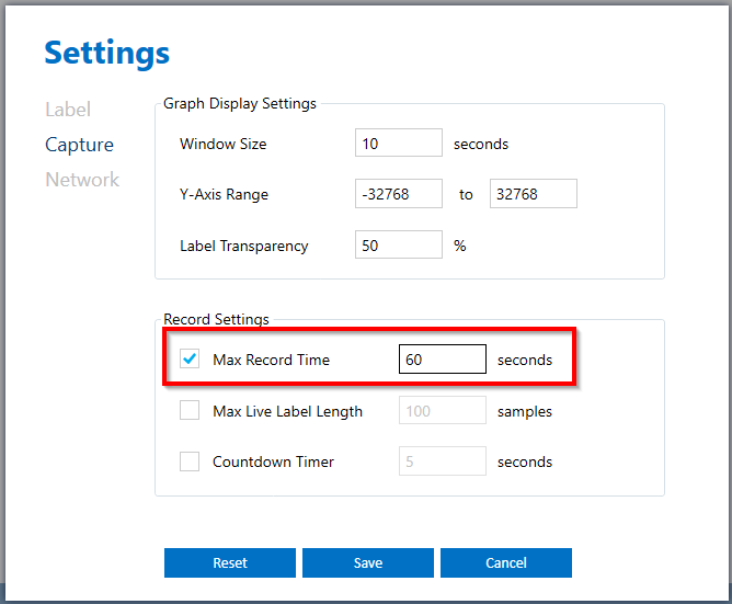
Once you are happy with the capture settings, click save and then press “Start Recording”. We recommend you record only one specific event per recording and name your captured files accordingly. This makes it easier to organize your files and find audio events that are mislabeled.
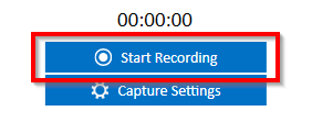
Note that you can finish each recording before the designated time by pressing Stop Recording. If you have not set any maximum limit for your recording, you can continue capturing data for any arbitrary time.
TIPS
Leave silent space (around 1/2 second) between different audio events. For instance, if you are recording a Locking event, wait for some time before you turn the doorknob or the key. If you repeat an action several times and quickly, it would be much harder to distinguish various events and annotate the data
Try to change the speed of an audio event. For instance, if you are inserting a key into the keyhole, do it at fast and gentle speeds.
If you are recording knocking events, try to include single knocks and a chain of multiple knocks. Leave enough space between singles and multiples to make it more clear when an event starts and ends.
Try to be consistent when generating and recording audio event, i.e. do not introduce extra noise or do not make any additional movements such as unnecessary jiggling
Collect data for both training and validation/testing and name the capture files accordingly. This helps to have better control over the data flow and to make sure we do not end up testing our model with the same data (or segments of data) that originally used for building the model. Usually, the rule of thumb is to set aside ~25% of the recorded data for validation/testing purposes.
Preferably, collect data without other noise in the background. You always have the option to add noise later and augment your dataset
Data Annotation
Defining Labels
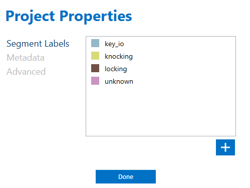
If you have not defined your desired labels on Data Studio, you can go to Top Menu> Edit> Project Properties and define as many labels as your project needs using the plus sign on the bottom right side of the window.
Defining a Session
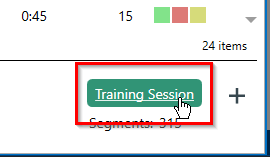
Before beginning the annotation process, you need to create an annotation session. In this tutorial we use the manual annotation method. To create a new session, click on the session name in the bottom right corner of the Project Explorer.
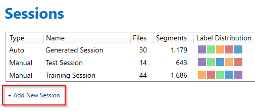
Click Add New Session
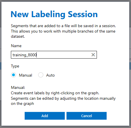
Choose Manual and name your session. Create two sessions, one for training and one for testing purposes.
Data Labeling
Known Classes
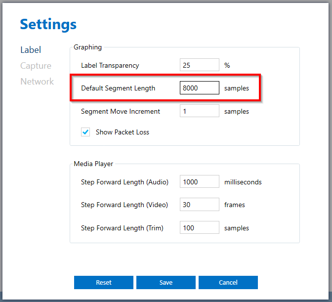
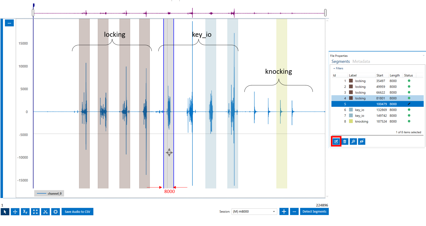
For this demo project, after some exploration we decided to use segments with the size of 8,000 samples (1/2 second). Change the default segment size by going to Top Menu> Edit> Settings> Label and set the Default Segment Length to 8,000 samples.
These are the steps to annotate your data:
On the top left corner of the Data Studio, click on the Project Explorer and open the capture file you want to annotate
You can listen to the capture file using the play button in the Media Player
Use your middle mouse wheel to zoom in/out
Right clicking on any part of the signal, generates a segment with the pre-defined size (e.g. 8,000 samples). Note that this segment does not have a label yet
You can move the segment you created by holding the left mouse key and dragging the segment to the right or left
Try your best to fit the entire audio event (or as much as possible) inside the segment
If you find out that you need larger segment sizes, you can change the default segment size by following the step we described above. Another option would be to drag the right or left border of the segment, once it is selected, and adjust the segment length
Select a segment (or multiple segments) and click on the edit button on the bottom left side of the Segment Explorer window to assign a label to your segment.
Unknown Classes
In order for this process to be successful, we need to collect some data that doesn’t fall into any of the desired categories. Having a variety of different noise data improves the performance of the model and helps the training algorithm converge faster.
These are some methods to collect noise data:
Collect street noise
Collect party noise
Search for YouTube videos to collect fan/shower/crowd noise
Including white/blue/pink noise is recommended
Labeling the noise data is fairly easy because there are not any meaningful parts of the data.
In this tutorial, we use almost the first ~2/3 part of the signal for training
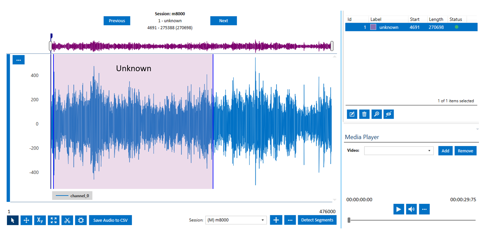
and the last ~1/3 is set aside for validation and testing.
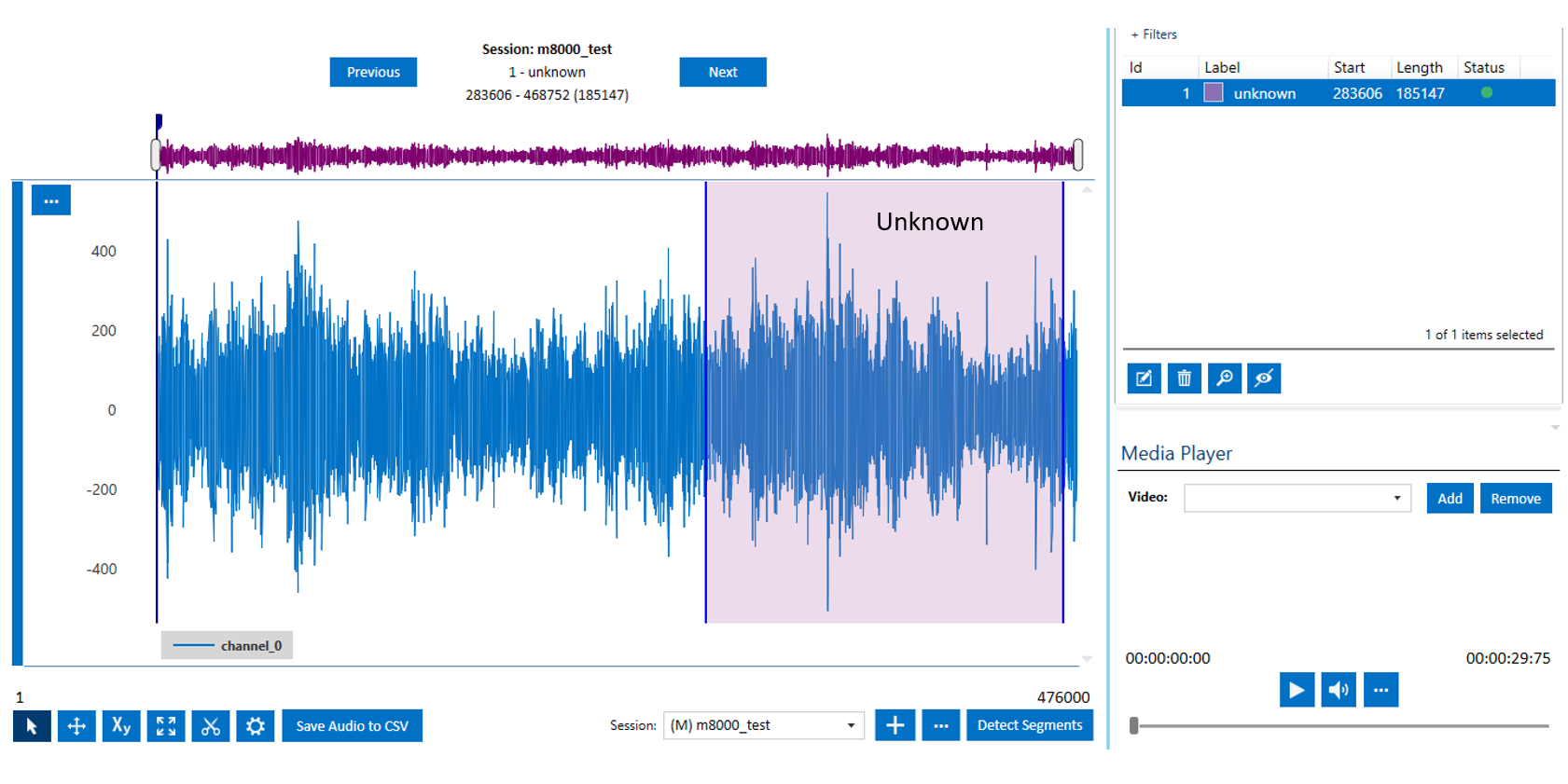
Note that the labelled region is much larger in the case of noise data. Later, the smaller segmented windows would be automatically extracted by the feature generation pipeline.
Once you are done labeling your data, you can move on to generating your first model.
Note: If you have collected data separately for training and testing, make sure that you either specify the difference as a Metadata property in your file or you can define different labeling sessions for each set. In this tutorial we use different sessions to distinguish our training and testing dataset. Also, it is highly recommended to collect data for only one type of audio event in each capture file to have a smoother workflow.
TIP: If you have collected a large dataset, we suggest you first label a fraction of your dataset and jump into building your model. During the modelling process, if necessary, it is easier to make further annotation adjustments as you do not have to repeat the entire segmentation/labeling process for the entire project. We suggest you only collect enough data to build a reasonable model and keep adding/collecting more data as you are aiming to improve your model performance.
Building a Training/Testing Query
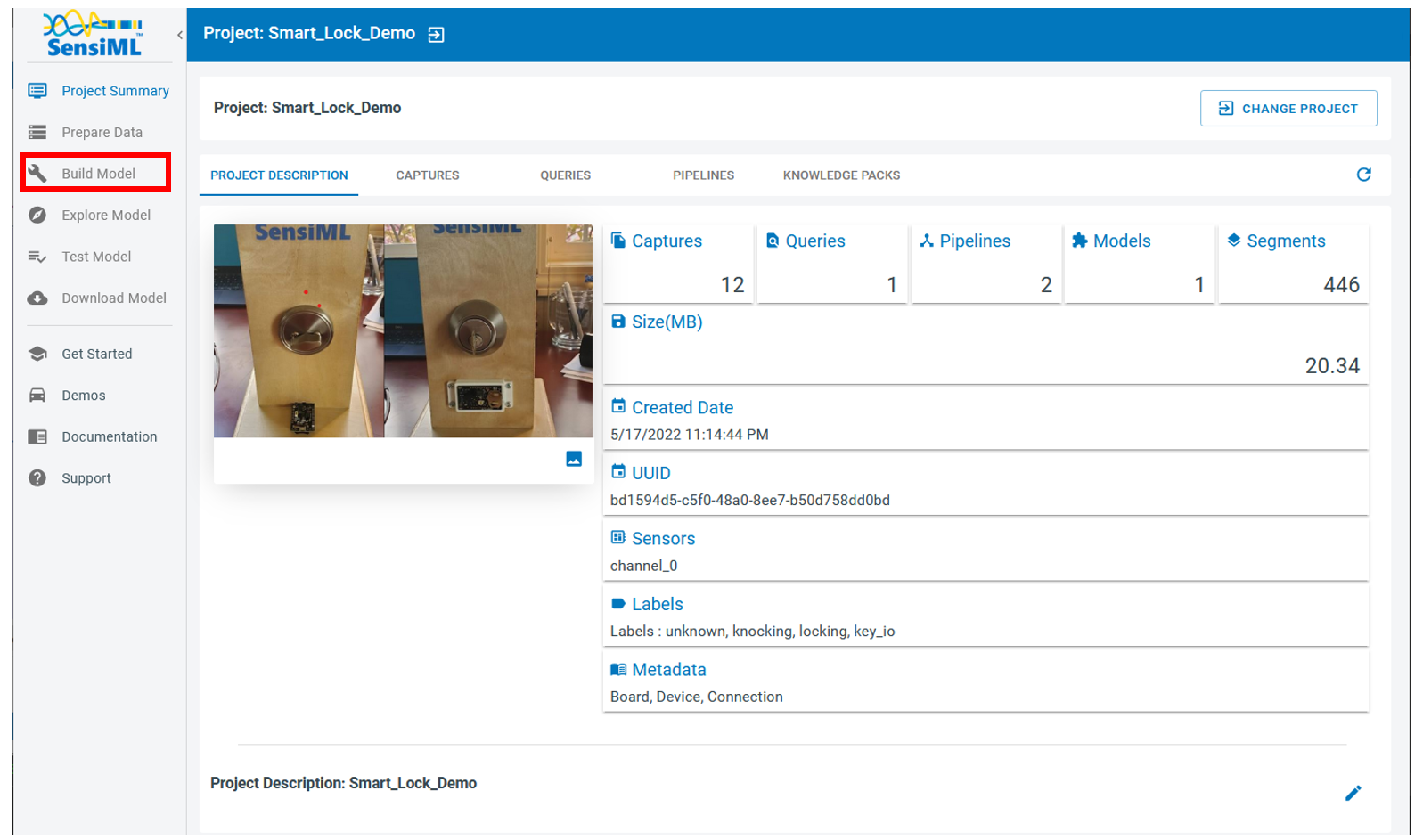
In this step, we generate queries to read and prepare the data in a format that is usable by the pipeline. In this tutorial we define queries using the SensiML Analytics Studio. Login to your account using the same credentials you used to create your project in the Data Studio.
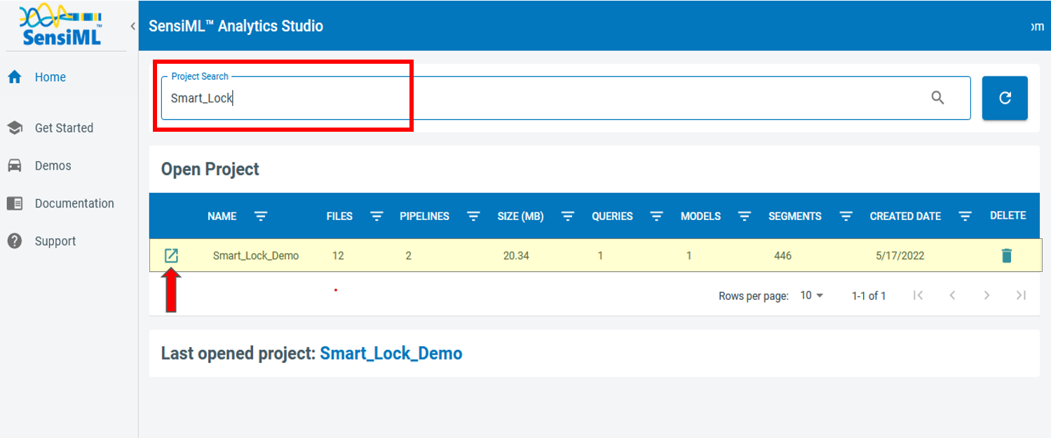
Once your project is loaded, you will be provided with general information about your project, such as the number of the captured files and total number of annotated segments, total number of queries, number of model training and feature generation pipelines, the number of models, and sensor names and other metadata.
Click on the Prepare Data on the left menu to add new queries
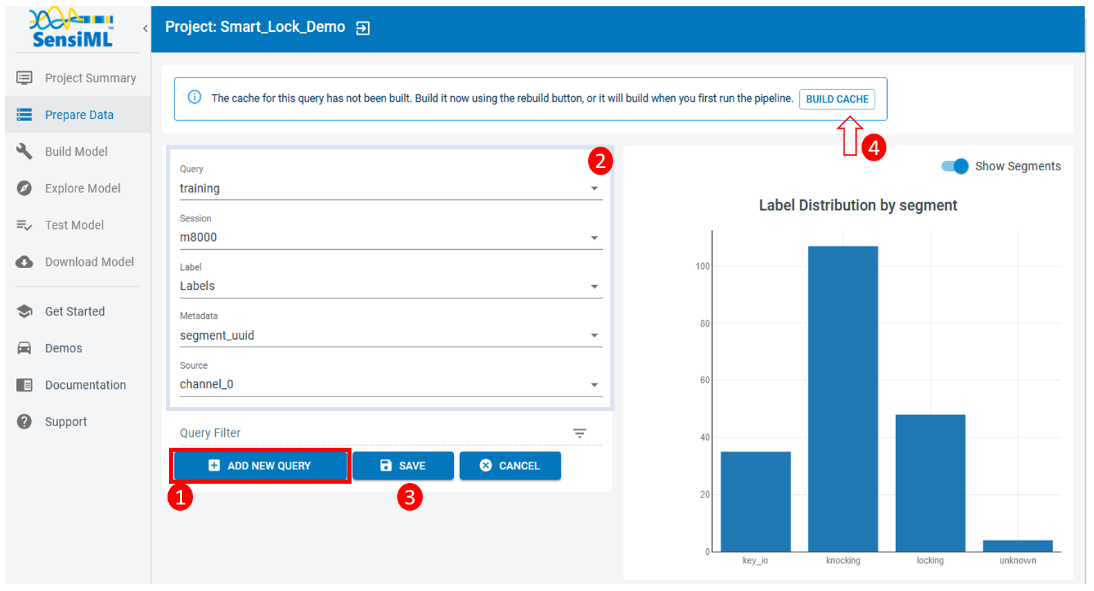
These are the steps you need to take to make a new query
Click on the “Add New Query” button
Fill in the form
2.1. Name your query based on the task you want to perform on the resulting data
2.2. Use the corresponding session name you defined on the Data Studio when annotating data. If you have two sessions for training and testing, here you need to repeat these steps and define two queries
2.3. Saving the query that basically saves the instructions to prepare your data
2.4. In order to execute the query and prepare data, you can click on the “Build Cache” button on the top right corner. Depending on how much data has been annotated in the corresponding session, this task may take several minutes to hours
TIP: On the bottom of the list, you have the chance to filter out your data based on some of the metadata columns on your project. Hence, if you have collected some meaningful metadata, you can query your data against those parameters
This is what you get once the execution of the query is completed
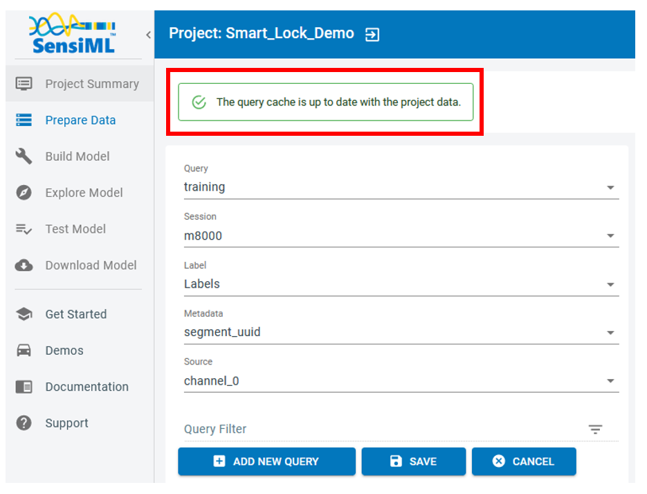
Whenever you add more annotated data to your project, you need to execute the query and stage the data.
You can also review the query list and check their latest status by selecting the Project Summary and opening the “QUERIES* tab
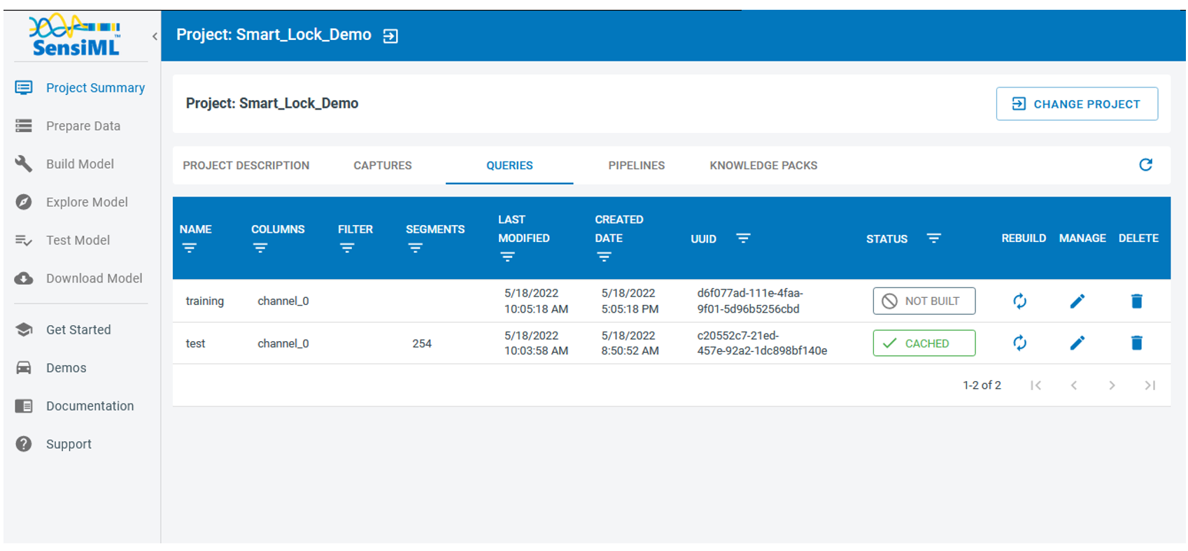
Note: In this project, we generate two queries, one for training and one for testing. We also make sure that training and testing segments are not overlapping.
Feature Extraction Pipelines
Setup
At this point we continue our work using the SensiML Python SDK. You won’t need to be a python expert or to be familiar with all the SDK functions. This tutorial walks through each step and provides all of the required commands.
If you do not have Python on your local machine, you can always use Google Colab to start a Jupyter Notebook instance on the Google cloud and follow along.
You are also welcome to use your own Jupyter Notebook/Lab instance from your local machine. However, the advantage of the Google Colab notebooks is that they already include most of the commonly used python packages.
Run the following cell to install the latest SensiML Python SDK.
!pip install sensiml -U
Importing Required Python Packages
from sensiml import *
import sensiml.tensorflow.utils as sml_tf
import os, sys
import os
os.environ['TF_CPP_MIN_LOG_LEVEL'] = '3'  # or any {'0', '1', '2'}
import numpy as np
import seaborn as sn
import matplotlib.pyplot as plt
import tensorflow as tf
from tensorflow.keras import layers
from tensorflow import keras
import math, warnings
warnings.filterwarnings('ignore')
Connecting to the SensiML Server
In this step, you connect to the SensiML server by providing your account credentials. Next, enter the name of your project.
dsk = SensiML()

dsk.project = "Smart_Lock_Demo"  # This is the name of your project
Data Exploration
Optional: This is another way to visualize the information you can find the Analytics Studio.
In the function get_query("query_name"), you need to enter the name of the query you previously generated in the Analytics Studio. In the next two cells, we quickly check the status of out training and testing queries.
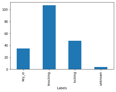
q = dsk.get_query("training")
q.statistics_segments().groupby('Labels').size().plot(kind='bar')
print(q.statistics_segments().groupby('Labels').size())
Labels
key_io       35
knocking    107
locking      48
unknown       4
dtype: int64
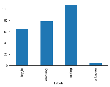
q = dsk.get_query("testing")
q.statistics_segments().groupby('Labels').size().plot(kind='bar')
print(q.statistics_segments().groupby('Labels').size())
Labels
key_io       65
knocking     78
locking     107
unknown       4
dtype: int64
Feature Generation Pipeline
In the following cells, we define a pipeline to generate features and then import the results to a local machine for building the model. In this method, we separately do feature generation and model training. Feature vectors are calculated in the SensiML server and the results will be transferred to your python client for further modelling analysis.
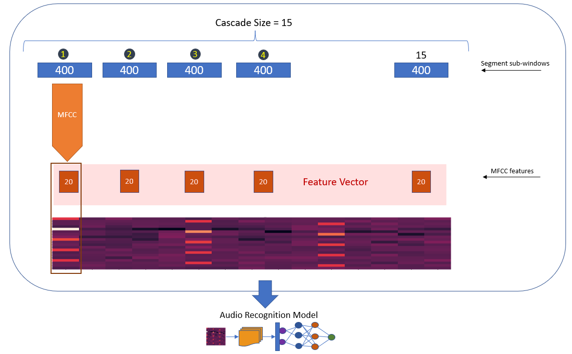
The following schematic graph displays how we build the feature vectors. First, we chop the time series data into windows of size 400 samples. Each of 400 samples will then be transformed through the Mel Frequency Cepstral Coefficients (MFCC) filter to extract significant characteristics of each segment in the frequency domain. Here, we extract 20 features out of each set of 400 samples. The generated vectors of 20 MFCC elements are combined using the feature cascading block. We set the cascade number to 15, that means each feature vector consists of 15x400=6,000 samples.
As mentioned earlier, most of the annotated segments of the target classes are of size 8,000. This means each segment with the length of 8,000 would turn into 5 individual segments of length 6,000, thus introducing a form of data augmentation. Moreover, this method helps with training of the convolutional layers that are responsible for extracting the shift-invariant features. Note that 6,000 is still large enough and covers the significant portion of the audio events we have considered.
Note that the length of segments, sub-windows, and the number of cascading features are all free parameters that require careful data exploration and analysis to set. The values that we have adopted here are justified for the current smart door lock application and may require extra tuning for other applications. In the classification mode, the sliding size is 400 sample, meaning that there is an inference after the collection of every 400 samples using the latest 6,000 samples. Thus, there would be 40 classifications in every second for the sample rate of 16 kHz.
This feature generation scenario is translated to Python as follows
n_mfcc=20         ### number of MFCC coefficients
cascade_size=15   ### number of features to cascade

def build_pipeline(dsk, query="query_name", pipeline="pipeline_name", undersample=False, energy_threshold=0, backoff=10):

    dsk.pipeline = pipeline
    dsk.pipeline.reset()

    dsk.pipeline.set_input_query(query, use_session_preprocessor=False )

    dsk.pipeline.add_transform("Windowing", params={"window_size": 400,
                                                    "delta": 400,
                                                    "train_delta": 0,
                                                    "return_segment_index": False,
                                                    })


    ## This is turned off when training
    ## It's only activated during classification
    dsk.pipeline.add_transform("Segment Energy Threshold Filter", params={"input_column":"channel_0",
                                    "threshold":energy_threshold,
                                    "backoff":backoff, "disable_train": True})


    # generating MFCC vectors
    dsk.pipeline.add_feature_generator([{'name':'MFCC', 'params':{"columns": ["channel_0"],
                                        "sample_rate": 16000,
                                        "cepstra_count": n_mfcc,
                                        }}])

    # combining feature vectors
    dsk.pipeline.add_transform("Feature Cascade", params={"num_cascades": cascade_size ,
                                    "slide": True,
                                    })

    ## This step randomly removes some of the more frequent labels to have even distribution over all labels
    ## Under-sampling helps to remove the model bias towards the more frequent labels
    if undersample:
        dsk.pipeline.add_transform("Undersample Majority Classes", params={"target_class_size":0,
                                        "maximum_samples_size_per_class":0,
                                        "seed":0})

    # this step scales the final feature vector to be compatible with 8-bit devices
    dsk.pipeline.add_transform("Min Max Scale", params={"min_bound": 0,
                                    "max_bound": 255,
                                    "pad": 0,
                                    "feature_min_max_defaults":{'minimum':-500000, 'maximum':500000.0},
                                    })

    return dsk
Feature Generation for Training Data
The following code snippet calls the function we defined above and runs it on the training query.
Here, the output of the training query used and mapped into the feature space. fv_train is a data frame that holds the pipeline output. feature_to_tensor is a function that adjusts the data frame and is capable of splitting the dataset into train/validate/test subsets.
The execution time of this pipeline depends on the size of the output data generated by the defined query. It may take between minutes to hours.
dsk = build_pipeline(dsk, query="training", pipeline="training", energy_threshold=0, backoff=14)


fv_train, s = dsk.pipeline.execute()

x_train, _, _, y_train, _, _,  class_map =  dsk.pipeline.features_to_tensor(fv_train, test=0, validate=0,
                                                                            shape=(-1, n_mfcc, cascade_size,1))
Executing Pipeline with Steps:

------------------------------------------------------------------------
 0.     Name: training                              Type: query
------------------------------------------------------------------------
------------------------------------------------------------------------
 1.     Name: Windowing                             Type: segmenter
------------------------------------------------------------------------
------------------------------------------------------------------------
 2.     Name: Segment Energy Threshold Filter               Type: transform
------------------------------------------------------------------------
------------------------------------------------------------------------
 3.     Name: generator_set                         Type: generatorset
------------------------------------------------------------------------
------------------------------------------------------------------------
 4.     Name: Feature Cascade                       Type: transform
------------------------------------------------------------------------
------------------------------------------------------------------------
 5.     Name: Min Max Scale                         Type: transform
------------------------------------------------------------------------
------------------------------------------------------------------------


Results Retrieved... Execution Time: 0 min. 7 sec.
-----  Summary  -----
Class Map:{'key_io': 0, 'knocking': 1, 'locking': 2, 'unknown': 3}
Train:
 total:  5578
 by class: [ 210.  642.  288. 4438.]
Validate:
 total:  0
 by class: [0. 0. 0. 0.]
Test:
 total:  0
 by class: [0. 0. 0. 0.]
# fv_train is pandas data frame
fv_train.head()
| gen_c0000_gen_0001_channel_0mfcc_000000 | gen_c0000_gen_0001_channel_0mfcc_000001 | gen_c0000_gen_0001_channel_0mfcc_000002 | gen_c0000_gen_0001_channel_0mfcc_000003 | gen_c0000_gen_0001_channel_0mfcc_000004 | gen_c0000_gen_0001_channel_0mfcc_000005 | gen_c0000_gen_0001_channel_0mfcc_000006 | gen_c0000_gen_0001_channel_0mfcc_000007 | gen_c0000_gen_0001_channel_0mfcc_000008 | gen_c0000_gen_0001_channel_0mfcc_000009 | ... | gen_c0014_gen_0001_channel_0mfcc_000015 | gen_c0014_gen_0001_channel_0mfcc_000016 | gen_c0014_gen_0001_channel_0mfcc_000017 | gen_c0014_gen_0001_channel_0mfcc_000018 | gen_c0014_gen_0001_channel_0mfcc_000019 | CascadeID | Labels | SegmentID | segment_uuid | __CAT_LABEL__ | |
|---|---|---|---|---|---|---|---|---|---|---|---|---|---|---|---|---|---|---|---|---|---|
| 0 | 175 | 120 | 133 | 128 | 120 | 122 | 123 | 124 | 125 | 142 | ... | 125 | 124 | 125 | 127 | 129 | 0 | key_io | 0 | 13984602-8918-44e3-8cda-79cffeb753f8 | 0 |
| 1 | 198 | 98 | 125 | 137 | 107 | 109 | 107 | 117 | 122 | 139 | ... | 122 | 129 | 127 | 130 | 128 | 1 | key_io | 0 | 13984602-8918-44e3-8cda-79cffeb753f8 | 0 |
| 2 | 200 | 94 | 105 | 133 | 130 | 120 | 113 | 119 | 129 | 142 | ... | 123 | 129 | 129 | 127 | 127 | 2 | key_io | 0 | 13984602-8918-44e3-8cda-79cffeb753f8 | 0 |
| 3 | 206 | 90 | 115 | 140 | 114 | 122 | 95 | 126 | 127 | 135 | ... | 125 | 131 | 126 | 129 | 129 | 3 | key_io | 0 | 13984602-8918-44e3-8cda-79cffeb753f8 | 0 |
| 4 | 208 | 87 | 121 | 126 | 117 | 117 | 113 | 127 | 118 | 132 | ... | 122 | 128 | 127 | 128 | 128 | 4 | key_io | 0 | 13984602-8918-44e3-8cda-79cffeb753f8 | 0 |
5 rows × 305 columns
Feature Generation for Test Data
Similar to what we did for the training dataset, the following code snippet calls the function we defined above and runs it on the testing query.
energy_thresholdis the minimum signal amplitude within the region of interest (i.e. segments that are formed by 15x400=6,000 samples) that triggers the classification algorithm
dsk = build_pipeline(dsk, query="testing", pipeline="testing", energy_threshold=600, undersample=True, backoff=14)

fv_validate, s = dsk.pipeline.execute()

x_validate, _, _, y_validate, _, _,  class_map =  dsk.pipeline.features_to_tensor(fv_validate, test=0, validate=0,
                                                                                  shape=(-1,n_mfcc, cascade_size,1))
Executing Pipeline with Steps:

------------------------------------------------------------------------
 1.     Name: training                              Type: query
------------------------------------------------------------------------
------------------------------------------------------------------------
 1.     Name: Windowing                             Type: segmenter
------------------------------------------------------------------------
------------------------------------------------------------------------
 1.     Name: Segment Energy Threshold Filter               Type: transform
------------------------------------------------------------------------
------------------------------------------------------------------------
 1.     Name: generator_set                         Type: generatorset
------------------------------------------------------------------------
------------------------------------------------------------------------
 1.     Name: Feature Cascade                       Type: transform
------------------------------------------------------------------------
------------------------------------------------------------------------
 1.     Name: Undersample Majority Classes          Type: sampler
------------------------------------------------------------------------
------------------------------------------------------------------------
 1.     Name: Min Max Scale                         Type: transform
------------------------------------------------------------------------
------------------------------------------------------------------------


Results Retrieved... Execution Time: 0 min. 1 sec.
-----  Summary  -----
Class Map:{'key_io': 0, 'knocking': 1, 'locking': 2, 'unknown': 3}
Train:
 total:  840
 by class: [210. 210. 210. 210.]
Validate:
 total:  0
 by class: [0. 0. 0. 0.]
Test:
 total:  0
 by class: [0. 0. 0. 0.]
Feature Visualization
This step is optional and does not affect the overall model building process
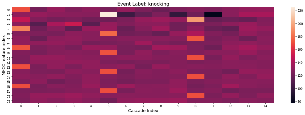
feature_array = fv_train[fv_train.columns[:-5]].values
event_index = 500
vector = feature_array[event_index].reshape((n_mfcc, cascade_size))

event_label = fv_train.Labels.iloc[event_index]


plt.figure(figsize=(20,6))
sn.heatmap(vector)
plt.xlabel("Cascade Index", fontsize=14)
plt.ylabel("MFCC feature index", fontsize=14)
plt.title("Event Label: "+event_label, fontsize=16)
Text(0.5, 1.0, 'Event Label: knocking')
TensorFlow Model
We use TensorFlow to implement our Convolutional Neural Network that takes the 1-dimentional feature vector and treats it a 2-dimentional image, similar to the plot displayed above.
The number of convolutional layers and their sizes have been optimized by trial and error. Therefore, the current network setup does not necessarily reflect the best possible architecture. Our main objective is the trainability (the ability of the algorithm to converge) and avoiding over-fitting.
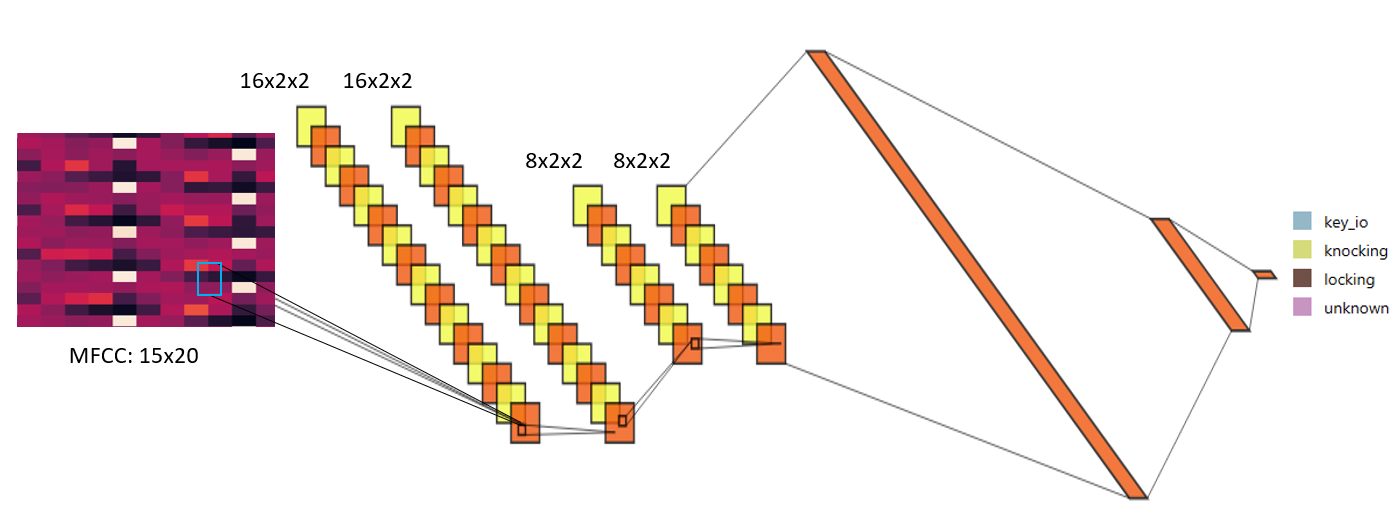
This network benefits from 4 sets of convolutional layers and two fully connected layers. You can play with this architecture to change the complexity and the number of free parameters that would be determined during the training process.
Model Definition
In the following block we implement the network the illustrated network in python. The network summary and the number of parameters are listed below.
optimization_metric = "accuracy"

tf_model = tf.keras.Sequential()

# input layer
tf_model.add(keras.Input(shape=(x_train[0].shape[0], x_train[0].shape[1], 1)))

# convolutional layers #1
tf_model.add(layers.Conv2D(16, (2,2), padding="valid", activation="relu"))
tf_model.add(layers.Dropout(0.25))
tf_model.add(layers.Conv2D(16, (2,2), padding="valid", activation="relu"))

# avoding overfitting
tf_model.add(layers.BatchNormalization(axis = 3))
tf_model.add(layers.Dropout(0.25))

# convolutional layers #2
tf_model.add(layers.Conv2D(8, (2,2), padding="valid", activation="relu"))
tf_model.add(layers.Dropout(0.25))
tf_model.add(layers.Conv2D(8, (2,2), padding="valid", activation="relu"))

# fully connected layers
tf_model.add(layers.Flatten())
tf_model.add(layers.Dense(16, activation='relu', ))

tf_model.add(layers.Dense(len(class_map.keys()), activation='softmax'))
tf_model.compile(optimizer='Adam', loss='categorical_crossentropy', metrics=[optimization_metric])

tf_model.summary()
Model: "sequential"
_________________________________________________________________
 Layer (type)                Output Shape              Param #
=================================================================
 conv2d (Conv2D)             (None, 19, 14, 16)        80

 dropout (Dropout)           (None, 19, 14, 16)        0

 conv2d_1 (Conv2D)           (None, 18, 13, 16)        1040

 batch_normalization (BatchN  (None, 18, 13, 16)       64
 ormalization)

 dropout_1 (Dropout)         (None, 18, 13, 16)        0

 conv2d_2 (Conv2D)           (None, 17, 12, 8)         520

 dropout_2 (Dropout)         (None, 17, 12, 8)         0

 conv2d_3 (Conv2D)           (None, 16, 11, 8)         264

 flatten (Flatten)           (None, 1408)              0

 dense (Dense)               (None, 16)                22544

 dense_1 (Dense)             (None, 4)                 68

=================================================================
Total params: 24,580
Trainable params: 24,548
Non-trainable params: 32
_________________________________________________________________
2022-05-18 23:34:47.210471: E tensorflow/stream_executor/cuda/cuda_driver.cc:271] failed call to cuInit: UNKNOWN ERROR (100)
2022-05-18 23:34:47.210530: I tensorflow/stream_executor/cuda/cuda_diagnostics.cc:156] kernel driver does not appear to be running on this host (PW5530-EKOURKCH): /proc/driver/nvidia/version does not exist
2022-05-18 23:34:47.211067: I tensorflow/core/platform/cpu_feature_guard.cc:151] This TensorFlow binary is optimized with oneAPI Deep Neural Network Library (oneDNN) to use the following CPU instructions in performance-critical operations:  AVX2 FMA
To enable them in other operations, rebuild TensorFlow with the appropriate compiler flags.
Model Training
In the following block, we train the model by calling the fit function. Some of the free parameters are
n_epoch: Number of training iterations. Adjust this value if the training algorithm has not yet converged. You can test this by looking at the metric plots and evaluate how the accuracy metric evolves as the training goes on.
batch_size: Choose a number (should be preferably power of 2) between 16 and 128. Sometimes smaller number help to avoid the bias and false positive rate
shuffle: Set this boolean to True if you want to shuffle the training data set over the batches before each training epoch starts. Note: Batch normalization and dropout layers are activated during the training episodes and not during the testing/validation. These layers are not trainable and just prevent over-fitting.
n_epoch = 5
batch_size = 64
shuffle = True
from IPython.display import clear_output
train_history = {'loss':[], 'val_loss':[], 'accuracy':[], 'val_accuracy':[]}
history = tf_model.fit(x_train, y_train,
epochs=n_epoch,
batch_size=batch_size,
validation_data=(x_validate, y_validate),
verbose=1, shuffle=shuffle)
for key in train_history:
train_history[key].extend(history.history[key])
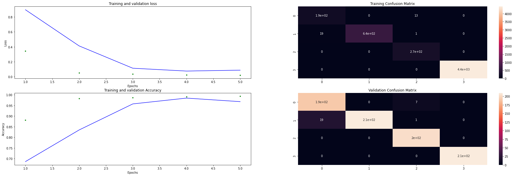
# plotting the training/validation metrics in terms of epoch number
sml_tf.plot_training_results(tf_model, train_history, x_train, y_train, x_validate, y_validate)
Epoch 1/5
88/88 [==============================] - 33s 370ms/step - loss: 0.3455 - accuracy: 0.8813 - val_loss: 0.8956 - val_accuracy: 0.6857
Epoch 2/5
88/88 [==============================] - 2s 22ms/step - loss: 0.0522 - accuracy: 0.9823 - val_loss: 0.4120 - val_accuracy: 0.8345
Epoch 3/5
88/88 [==============================] - 2s 21ms/step - loss: 0.0342 - accuracy: 0.9871 - val_loss: 0.1134 - val_accuracy: 0.9571
Epoch 4/5
88/88 [==============================] - 2s 23ms/step - loss: 0.0255 - accuracy: 0.9907 - val_loss: 0.0755 - val_accuracy: 0.9845
Epoch 5/5
88/88 [==============================] - 2s 27ms/step - loss: 0.0201 - accuracy: 0.9937 - val_loss: 0.0875 - val_accuracy: 0.9679
Post-Training Quantization
We need to quantize the model to fit in an 8-bit device prior to building the firmware. The following cell takes the tensor that defines our model and uses the TensorFlow Lite optimizer to convert it to a quantized format that is compatible with tiny devices.
The input of the cell is tf_model and the quantized version is called tflite_model_quant.
You don’t need to play with the following code. The only option that you have is to change the converter optimization algorithm. The options are:
tf.lite.Optimize.DEFAULTtf.lite.Optimize.EXPERIMENTAL_SPARSITYtf.lite.Optimize.OPMIZE_FOR_LATENCYtf.lite.Optimize.OPTIMIZE_FOR_SIZE
Note that all of the optimizations have pros and cons. For instance, you may find optimizing for latency negatively affects the model performance and vice versa.
def representative_dataset_generator():
    for value in x_train:
        yield [np.array([value], dtype=np.float32)]

# Unquantized Model
converter = tf.lite.TFLiteConverter.from_keras_model(tf_model)
tflite_model_full = converter.convert()
print("Full Model Size", len(tflite_model_full))

# Quantized Model
converter = tf.lite.TFLiteConverter.from_keras_model(tf_model)
converter.optimizations = [tf.lite.Optimize.DEFAULT]

converter.target_spec.supported_ops = [tf.lite.OpsSet.TFLITE_BUILTINS_INT8]
converter.inference_input_type = tf.int8
converter.inference_output_type = tf.int8

# converter.experimental_new_converter = False
converter.representative_dataset = representative_dataset_generator
tflite_model_quant = converter.convert()

print("Quantized Model Size", len(tflite_model_quant))
Now we can upload the quantized version of our model, i.e. tflite_model_quant to the SensiML server.
Here, we add our model to the end of the validation pipeline that we originally used to extract the features of the validation dataset. We set the training algorithm to Load Model TF Micro and pass the quantized tensor to the pipeline.
Execution of this pipeline uploads the model and tests the results against the validation set. This is because we are using the prepared data from the testing query.
The model that we have generated generates classifications in the form of a 1-dimensional array, whose elements are between 0 and 1 and all add up to 1.
For instance, if the class map is defined as Class Map:{'key_io': 0, 'knocking': 1, 'locking': 2, 'unknown': 3} then the returned class-vector would be a 4-dimentional array. For instance, (0.85, 0.05, 0.04, 0.01) means that there is a 85% likelihood that the classified segment belongs to a knocking event.
If the following block, we can set a threshold above which we call the classification robust. In cases of unknown signals, the classification vector falls in one of the following categories
The fourth element of the output class is largest and close to 1
None of the outputs are close to 1 and below the specified threshold, say 85%. In that case, an unsuccessful classification has been made and most likely the corresponding segment belongs to a signal that has not yet been observed by the neural network, or in general falls into the Unknown class.
class_map_tmp = {k:v+1 for k,v in class_map.items()} #increment by 1 as 0 corresponds to unknown

dsk.pipeline.set_training_algorithm("Load Model TF Micro",
                                    params={"model_parameters": {'tflite': sml_tf.convert_tf_lite(tflite_model_quant)},
                                            "class_map": class_map_tmp,
                                            "estimator_type": "classification",
                                            "threshold": 0.80, # must be above this value otherwise is unknown
                                            "quantization": "int8"
                                            })

dsk.pipeline.set_validation_method("Recall", params={})

dsk.pipeline.set_classifier("TF Micro", params={})

dsk.pipeline.set_tvo()

results, stats = dsk.pipeline.execute()
Confusion Matrix
In the following cell we extract the confusion matrix based on the validation set.
UNK stands for Unknown unknowns, where all elements of the class matrix are below the specified threshold, (which has been set to 80% in this tutorial).
model = results.configurations[0].models[0]
model.confusion_matrix_stats['validation']
CONFUSION MATRIX:
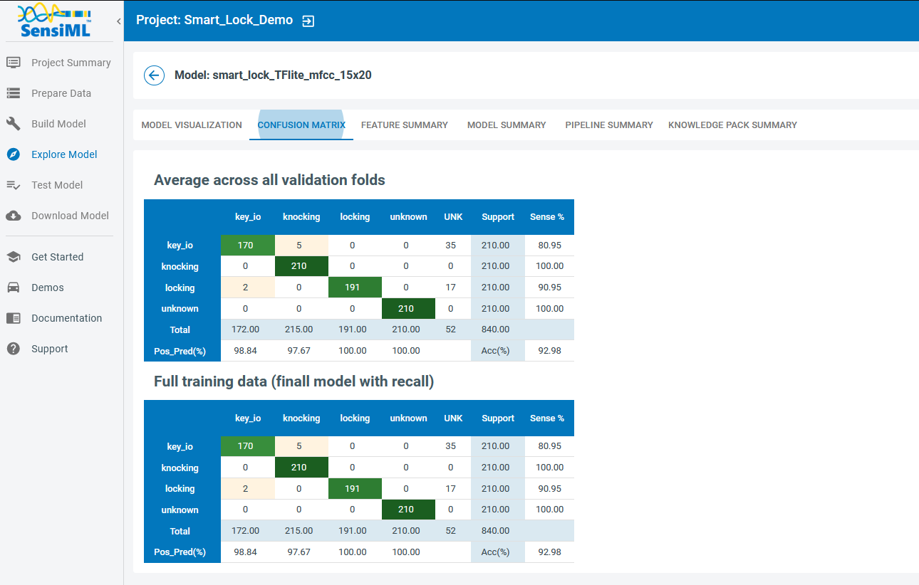
key_io knocking locking unknown UNK UNC Support Sens(%)
key_io 170.0 5.0 0.0 0.0 35.0 0.0 210.0 81.0
knocking 0.0 210.0 0.0 0.0 0.0 0.0 210.0 100.0
locking 2.0 0.0 191.0 0.0 17.0 0.0 210.0 91.0
unknown 0.0 0.0 0.0 210.0 0.0 0.0 210.0 100.0
Total 172 215 191 210 52 0 840
PosPred(%) 98.8 97.7 100.0 100.0 Acc(%) 93.0
You can also check out the confusion matrix and other model characteristics in the Analytics Studio, following the Explore Model menu option, under the Confusion Matrix tab.
Saving the Model
Eventually, if we are satisfied with the model performance and the extracted metrics, we save it on the server. This model can be later converted to Knowledge Packs for testing live on the Data Studio or for deploying on the desired edge devices
_ = model.knowledgepack.save("smart_lock_TFlite_mfcc_15x20")
Knowledgepack 'smart_lock_TFlite_mfcc_15x20' updated.
Running a Model in Real-Time in the Data Studio
Before downloading the Knowledge Pack and deploying it on the device, we can use the Data Studio to view model results in real-time with your data collection firmware.
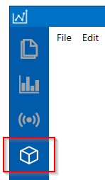
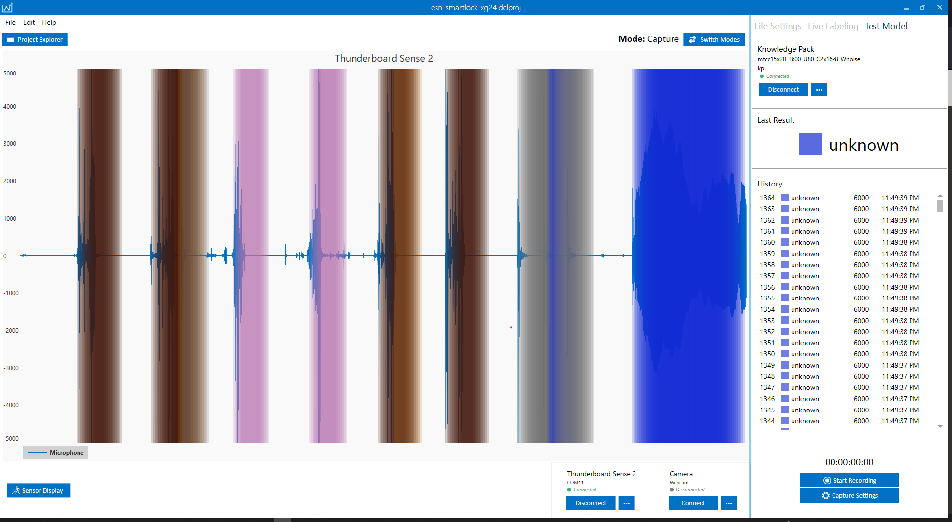
Open the Data Studio and open Test Model mode by clicking the Test Model button in the left navigation bar. Make sure that the data capture firmware is still running on your device.
Connect to your device
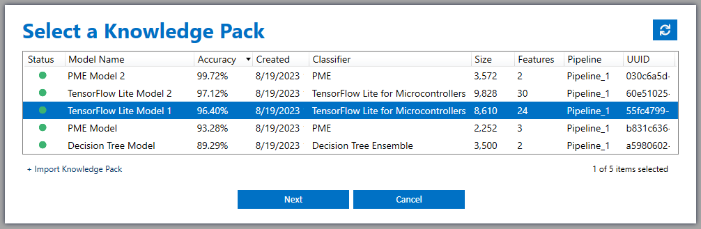
Connect to the Knowledge Pack you created above.
Select a session for the live streaming. In general, you can define a manual labeling session and call it KP and use it in the live streaming mode.
Once the Data Studio connects to your model, it generates inferences as it streams the data. Since we set the energy threshold to a value larger than the typical ambient noise level (say 600), the classification does not necessarily happen during the entire audio streaming.
Use your key and the doorknob to generate your events of interest and observe how the model performs
Live streaming mode is a powerful tool to evaluate the model performance and is good for collecting more data to augment your dataset.
Download/Flash the Model Firmware
In the analytics Studio, go to the Download page from the left menu bar.
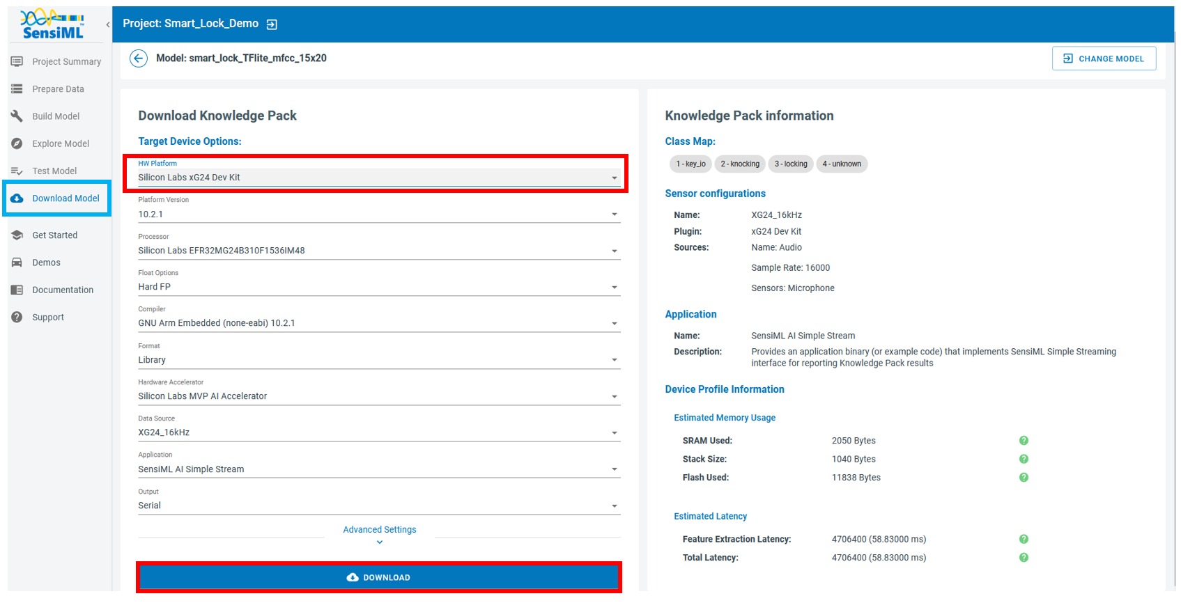
Select your device and press the Download button. Once the Knowledge Pack is download follow the corresponding instruction for your device here to flash the firmware.
Running a Model in Real-Time on a Device
You can download the compiled version of the Knowledge Pack from the Analytics Studio and flash it to your device firmware.
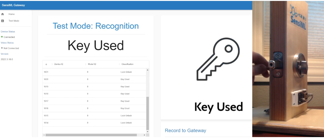
To see classification results, you may use a terminal emulator such as Tera Term or the Open Gateway.
For additional documentation please refer to the Running a Model on Your Embedded Device Documentation.
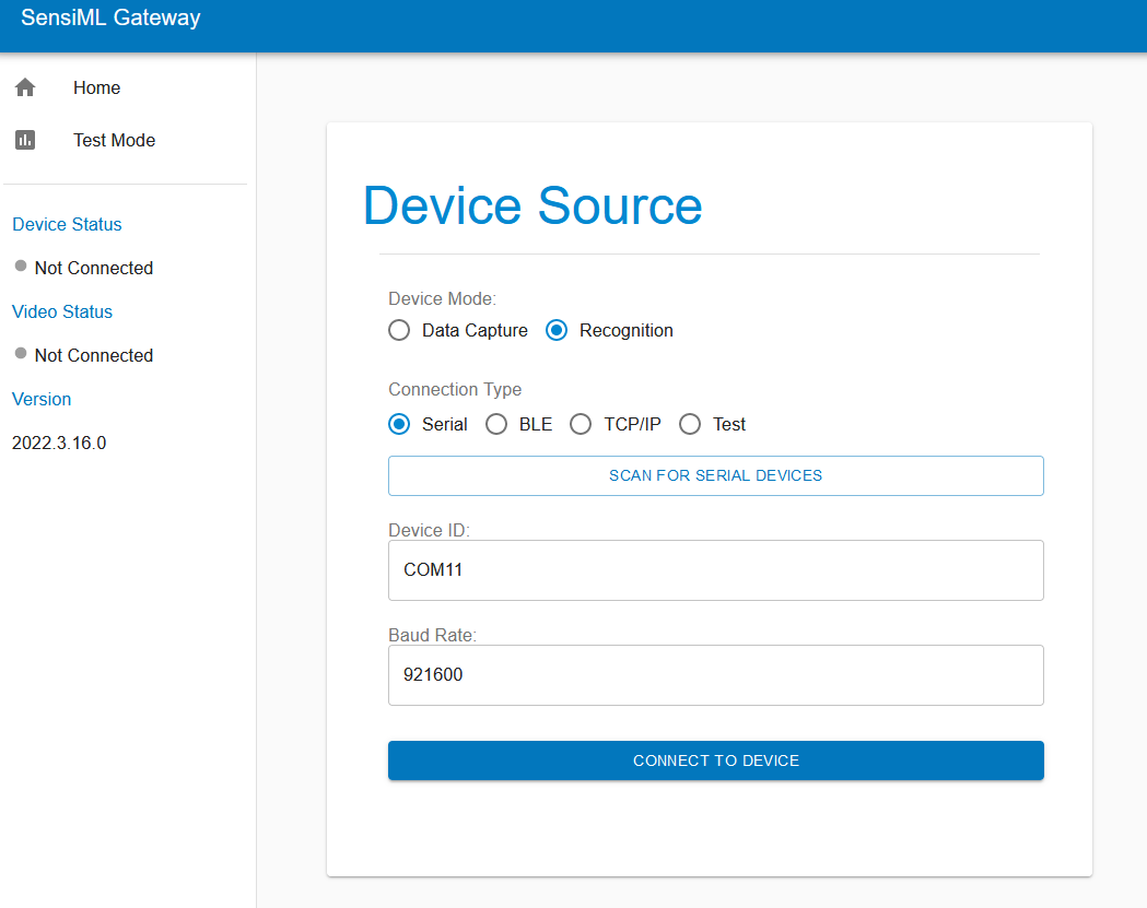
Open the Open Gateway and select Device Mode: Recognition and Connection Type: Serial. Scan for the correct COM port and set the baud rate to 921600. Next, click Connect To Device.
Switch to Test mode, click the Upload Model JSON button and select the model.json file from the Knowledge Pack.
Set the Post Processing Buffer slider somewhere between 5 and 10 and click the Start Stream button. The Open Gateway will now start displaying the model classifications from the device in real-time.