Keyword Spotting
Overview
This tutorial is a step-by-step guide on how to build keyword spotting applications using the SensiML keyword spotting pipeline. Keyword spotting is a technique used to recognize specific words or phrases in audio signals, usually with the intent of triggering an action. It is used for recognizing commands, allowing users to control a device or application by speaking predetermined commands. For example, a keyword spotting system might be used to control a smart home device by recognizing specific commands like “turn on the light” or “play music”. Keyword spotting algorithms are often used in voice-enabled applications, such as voice-activated assistants, smart speakers, and interactive customer service. Other applications involve detecting acoustic events, such as baby’s cry or coughs, or identifying the speaker characteristics, such as gender or age. Keyword spotting algorithms can identify speech in noisy environments, such as a crowded room or outdoors. They can be used in wake word applications too. These types of application are primarily used in smart home devices. Most home edge devices remain in hibernating mode to conserve energy. When the wake word is heard, the device becomes activated and responds to extra voice commands and/or runs complicated tasks.
The process of keyword spotting typically involves breaking down the audio signal into a series of small, overlapping windows, and then applying a signal processing technique such as a Fast Fourier Transform (FFT) to each window. This will convert the audio signal from the time domain into the frequency domain, to extract relevant features from the audio signal. These features are then passed through a machine learning algorithm, in this case, a deep convolutional neural network, to identify keywords. The neural network is trained using a labeled dataset of audio samples containing the keywords, and without. Once trained, the network can be used to predict whether the keyword or phrase is present within the provided frame of audio signal.
Objectives
This instruction shows how to build a keyword spotting model that identifies four keywords, i.e. “On”, “Off”, “Yes” and “No”. The major steps are
Data Collection. You will need to collect audio samples for the keywords you want to detect. The audio data condition must meet all requirements of the desired application. For examples, the audio quality should match the condition of the deployment environment, such as but not limited to, the audio amplitude, background noise level, user gender, and diversity of the speakers. The collected audio sample must fairly represent the real-world scenario.
Data Annotation. Each segment of the audio signal that covers a specific keyword must be labelled accordingly.
Training. Once the data is fully annotated, you will train a model offered by one of the SensiML keyword spotting templates. Each template loads a neural network which is pre-trained using the Google speech command dataset. Adopting the transfer learning approach, the training process re-tunes some of the network parameters to accommodate the keywords of your dataset.
Testing/Evaluating. You will need to evaluate the trained model to make sure it is detecting the keywords accurately. To do this, you can use a test set of audio samples that you set aside from the beginning for this purpose.
Deploying. You flash the model to the edge device of interest. If you are satisfied with the accuracy of the generated model, you can compile it, download it and deploy it on your application device. Once the model is deployed, it is important to monitor its performance and accuracy in the production environment. If the model accuracy does not meet the requirements, you can iteratively revisit previous steps, for instance collecting additional data in a more realistic environment, and/or adjusting the training parameters.
Required Software/Hardware
This tutorial uses the SensiML Toolkit to manage collecting and annotating sensor data, creating a sensor preprocessing pipeline, and generating the firmware. Before you start, sign up for the free SensiML Community Edition to get access to the SensiML Analytics Toolkit.
Software
SensiML Data Studio (Windows 10) to collect and label the audio data.
SensiML Analytics Studio for data preparation and managing pipelines. This interface enables you to generate an appropriate Knowledge Pack for deployment on any of the supported devices.
Optional: SensiML Open Gateway or Putty/Tera Term to display the model classifications in real-time.
Hardware
Select from our list of supported platforms.
Use your own device by following the documentation for custom device firmware.
Note
Although this tutorial is agnostic to the chosen edge device, due to the complexity of the generated model, some devices might not have enough memory to store the model or generate classifications in a reasonable time. Devices with the capability of accelerating the matrix arithmetic operations are recommended, but not necessary.
Collecting Data
Starting with the Data Studio
We use Data Studio (install) in order to connect to the audio sensor and to collect data. If you have already collected your audio data, you can follow these steps to import your captured data into the SensiML server. If you are about to collect new data, please first consult with the Supported Devices section in the left menu bar of the SensiML documentation and flash the proper Data Collection Firmware to the device. If you don’t find your device in the list, please refer to this page to learn how to integrate your data into the Data Studio.
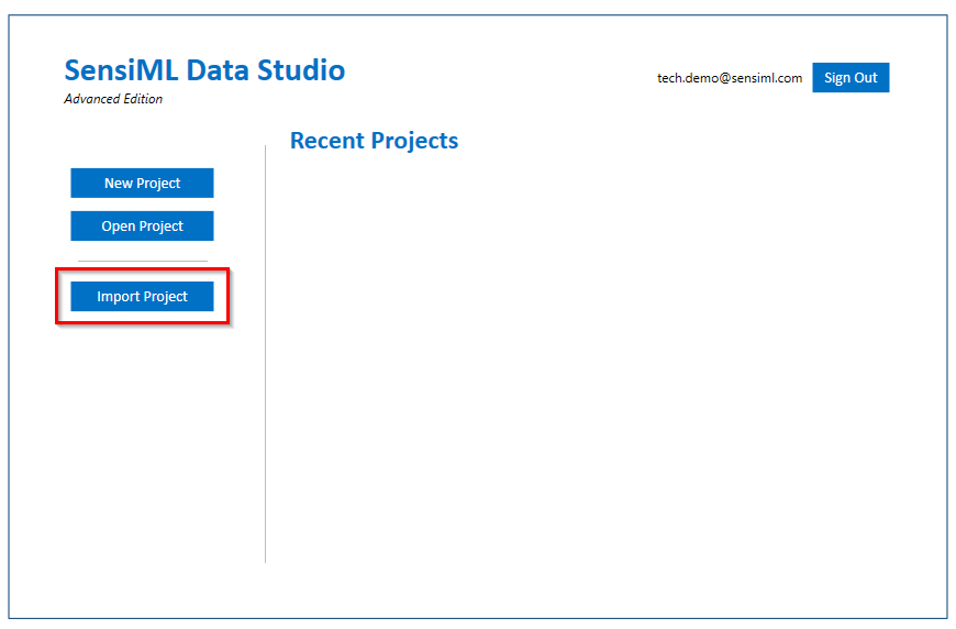
As an example, we have collected some data and stored them in a SensiML project. Follow the steps below to import the project to your account.
Download the example project
Import the project to your account using the Data Studio.
This project includes an example dataset of WAV files and four labels to represent keywords, “On”, “Off”, “Yes” and “No” as well as the additional label “Unknown” which is reserved for background noise and any other audio that does not include the known keywords.
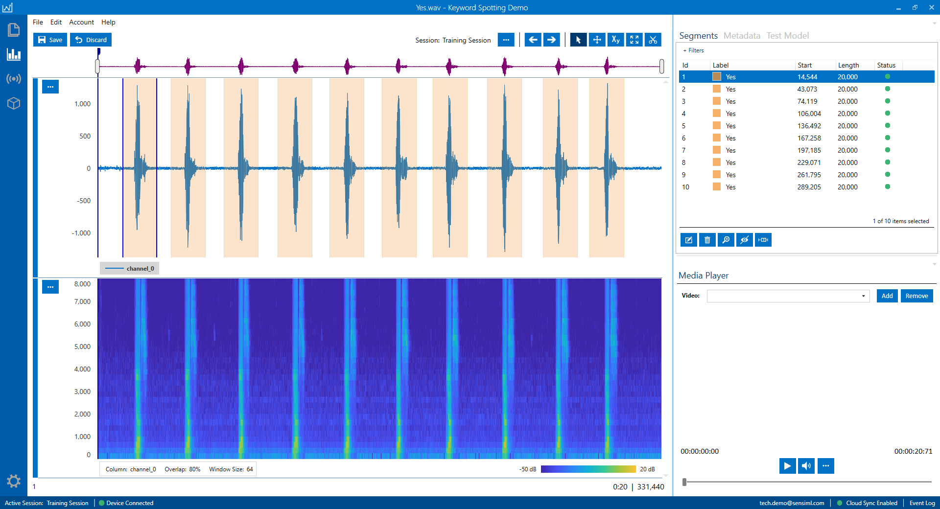
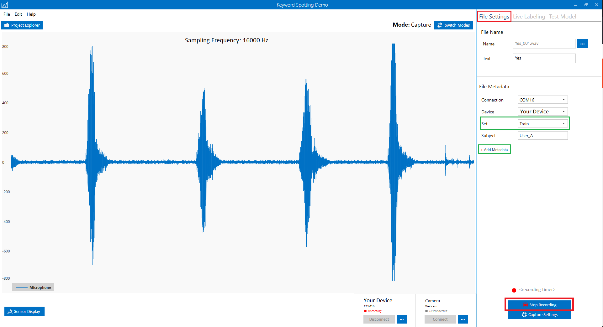
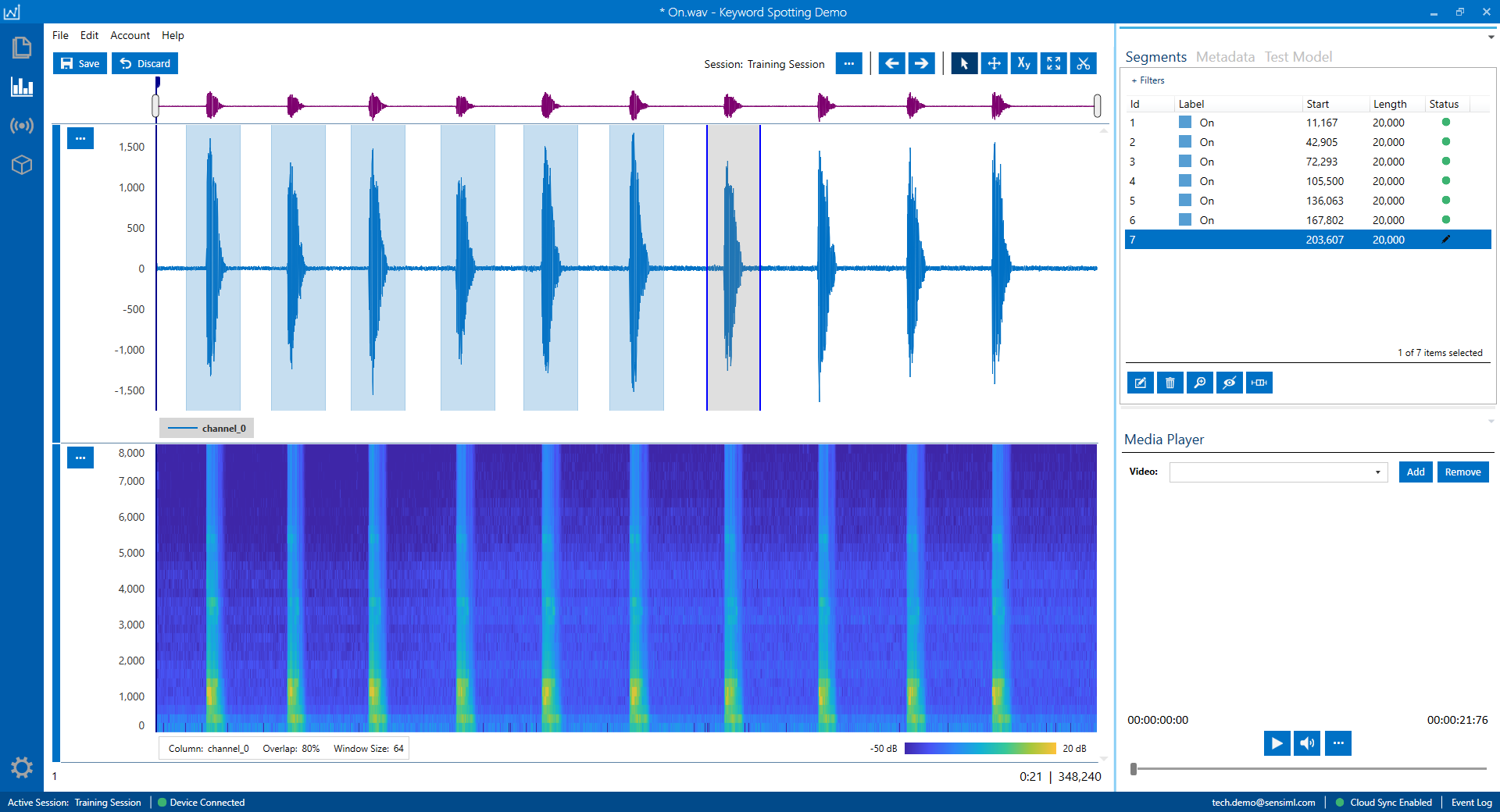
In the next image, you can see one of the WAV files displayed in the Data Studio.
The upper track shows the audio signal in blue with the labelled segments highlighted in orange.
The lower track illustrates the corresponding audio spectrogram. Spectrogram is a visual representation of how the sound energy is distributed over different frequencies. It helps with identifying patterns, tracking changes over time, and to examining the frequency balance of an audio signal.
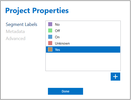
Note: The SensiML keywords spotting algorithm requires the audio dataset to include some data that are labelled as Unknown. The “Unknown” label must be exactly spelled the same way (i.e., in capitalized format). To see the list of labels, from the top menu of the Data Studio, click on Edit> Project Properties. You can click on the “+” sign to add new labels or right click on any of the labels to modify/delete them.
Recording Audio Data
We use Data Studio to connect to a device and collect audio data. Please also refer to this tutorial for further details on how to collect data using the Data Studio. Here, we briefly cover the main steps of data collection.
Note
Make sure that your device has been flashed with data collection firmware.
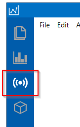
To collect new data, click on the Live Capture button in the left navigation bar
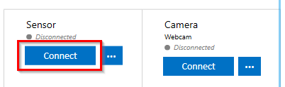
Now, we will prepare the Data Studio to communicate with the device and record data at the desired sampling rate. On the bottom of the Data Studio window, clicking on the Connect button, opens a window that allows you to scan your system. Find your device and adjust the capture settings (as explained here). The current SensiML keyword spotting models require the audio sampling rate to be 16000 Hz.
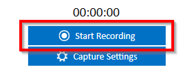
Once your device is connected to the Data Studio, the audio signal is displayed in real-time. At this point you can Start Recording the audio. You also have the option to adjust Capture Settings such as recording length, size and range of the display window.
If you are recording data for the keywords, leave enough space between the keyword events to experience a straightforward annotation later. To better track your workflow as you extend your dataset, it is recommended that each recording only include one keyword.
When you are done recording a file, click on the Stop Recording button and fill in the metadata form accurately.
We suggest you decide on the metadata fields before you start your data collection. You can add as many metadata fields as necessary.
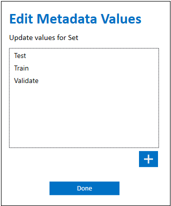
In this tutorial, we require uses to include a specific metadata field to keep track of data subsets. Usually 20-30% of the collected data is set aside for cross validation and testing purposes. Training data should not be taken in the validating and testing tasks. To make sure this condition always holds, we define a metadata field “Set” to store the category that the recorded data belong to. The Set column can take three values: “Train”, “Validate” and “Test”. By adding these options, we can guarantee the same data is never used for training, validation, and testing.
In this project, each recording belongs to only one Set and consists of one audio keyword.
If you are collecting data for multiple individuals, dedicate a separate metadata field to keep track of speakers.
Do not worry if you missed a few metadata fields and you want to introduce them later as your project evolves.
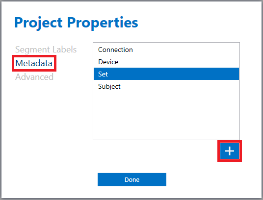
You always have the option to add, review, and modify metadata fields. To do so, from the main menu of the Data Studio click on Edit> Project Properties and go to the Metadata section. You can right click on any of the metadata items to delete/modify them or use the plus icon (+) to introduce new ones.
In this example, double clicking on “Set” opens the list of all possible options that will be accessible through a dropdown menu.
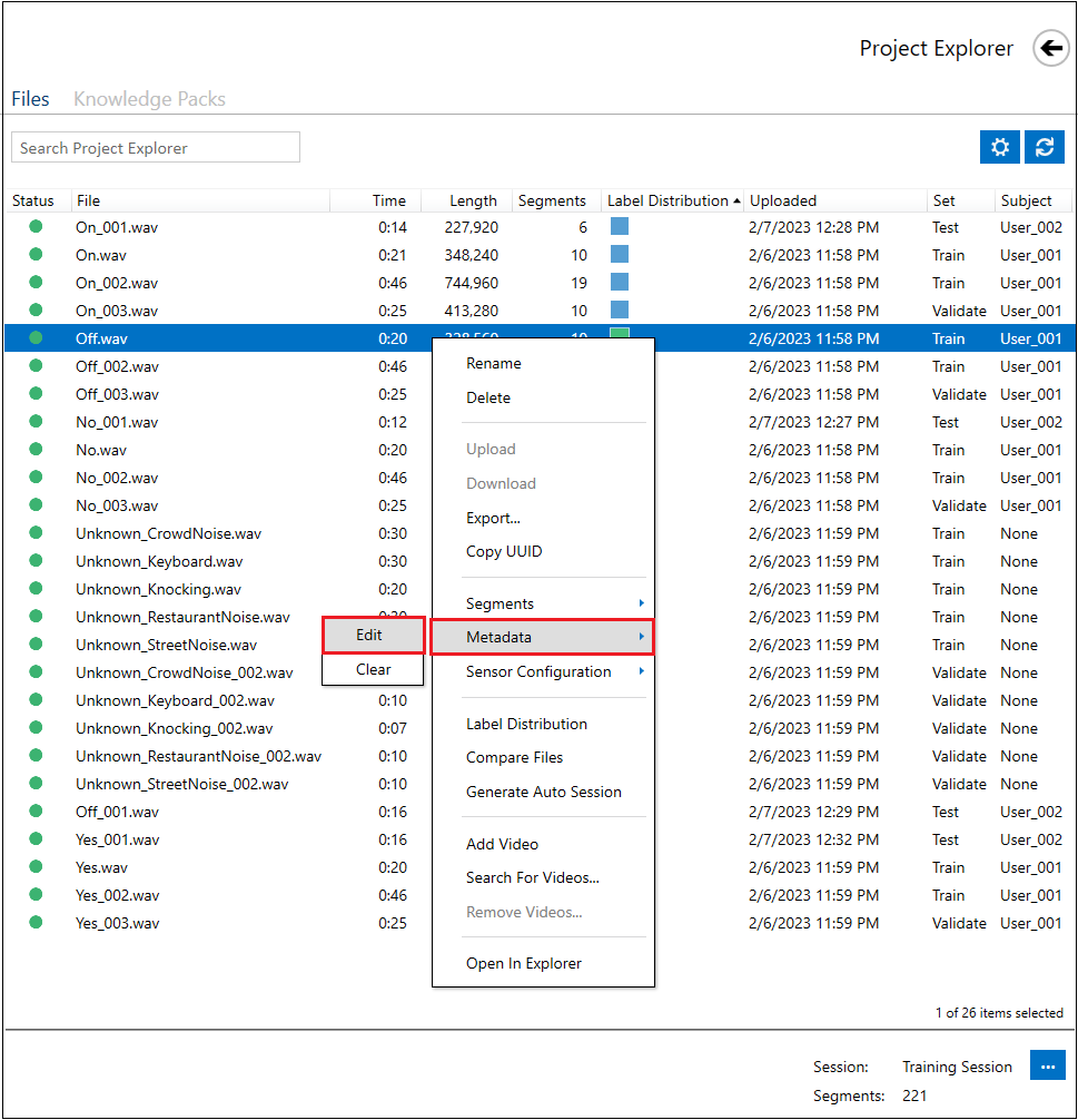
If you want to assign values to your newly defined metadata field of your previous recordings, or change their values, open the list of all recording by clicking on the “Project Explorer” on the top left, right click on the file name and select Metadata> Edit.
Data Annotation
Defining Labels
In case you have downloaded the example project, it already includes all four keyword labels (“Yes”, “No”, “On” and “Off”) plus the “Unknown” label for annotating audio noise and random speech events.
If you have created a new project for another set of keywords and have not yet defined your desired labels on the Data Studio, you can go to Top Menu> Edit> Project Properties and define as many labels as your project needs by using the plus icon (+) on the bottom right side of the window.
Defining Labeling Session
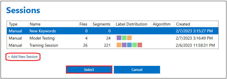
The Data Studio organizes label information in sessions. A session separates your labeled events (segments) into a group. This allows you to experience a better workflow with storing different versions of labels in separate sessions that can be later targeted by the data query block of the modeling pipeline. In order to make a new session, you can click on the session options button above the graph.
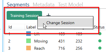
Click on “Add New Session” to create a new one. You can also switch between multiple labelling sessions.
Sessions can be leveraged in multiple ways. For instance, they can be used to keep track of the classifications made by various models on the same test data, or to store annotations produced by different protocols.
In this example, we used “Training Session” to store labels we use to build our keyword spotting model. We devote a separate session, “Model Testing”, to store the labels that are generated when testing a model.
Labeling the Audio Data
First, we switch to the labeling session we wish to use for training our model. Here, it is called “Training Session”.
Known Keywords
In this project, the keyword spotting model needs 1 second of the audio segment, consisting of 16,000 audio samples at the rate of 16 kHz. Don’t worry if the size of your keywords are slightly larger than 1 second. Our model is still capable of making reasonable classifications if a significant part of each keyword is covered within a 1-second data window.
Although each annotated segment of data must include at least 16,000 samples, we recommend increasing the size of segments by 25% and include about 20,000 samples in each segment. Here, the only condition is that every 16,000 subsegment must cover a significant part of the audio event. Segments that are smaller than 16,000 samples would not be considered in the model building process.
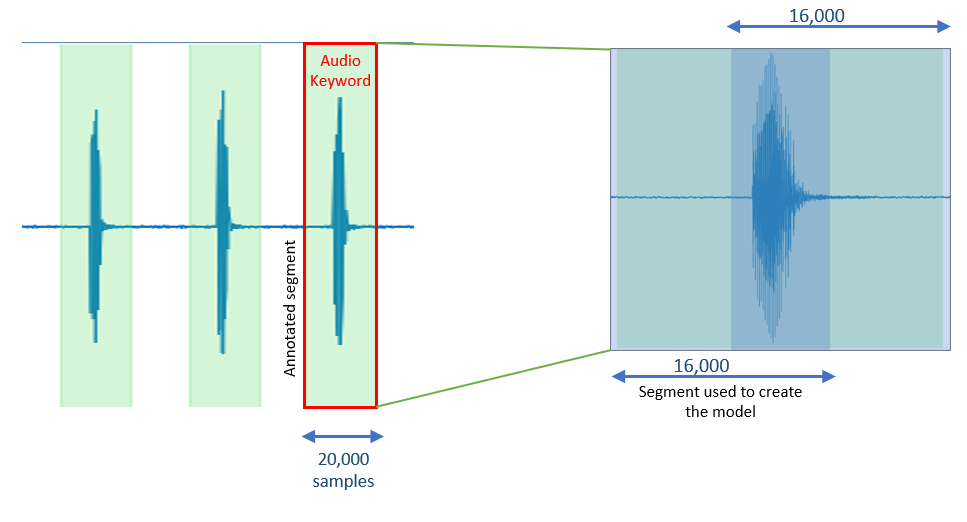
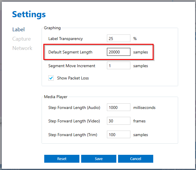
It is easier to set the default value of the segment size to a reasonable value. In this project, we set this value to be 20,000 samples.
Change the default segment size by going to Top Menu> Edit> Settings> Label and set the Default Segment Length to 20,000 samples.
Once you set the default segment size, open your keyword files, and label them accordingly.
To generate a new segment, right click on the signals where you want the segment to start. Try to place keywords at the center of segments.
Select the “Edit” button in the segment explorer box to change the label. By dragging the mouse pointer, you can also adjust the location and size of a selected segment.
During the data collection process, try to leave enough space between keywords to avoid overlapping segments. It is still acceptable of the edge of adjacent segments mildly overlap, as long the main body of the events are covered by different segments.
Unknown Audio Signals, Background Noise
As previously mentioned, in addition to the recording audio instances for each target keyword, you need to collect samples for variety of background noise conditions, such as traffic noise, room noise, and various types of ambient noise. We label these audio samples with the “Unknown” label. Having a good set of Unknown audio signals helps to improve the model accuracy by reducing the rate of false positive detection. In the context of an audio signal, this would mean that the signal is incorrectly classified as one of the model keywords while it belongs to a different random word or an environmental sound.
In this project, we consider two kinds of Unknown signals: (1) background noise and (2) random audio words.
For every project, the Unknown signals are carefully selected to address the project specifications. For most human keyword spotting applications, we suggest you include a good dataset of white/pink/blue random noise signals. You can simply play various environmental noise videos from the internet and capture the audio signal by your device. Few examples of interesting background noise that might influence the performance of any audio classification model are “fan noise”, “crowd noise”, “street noise”, “shower noise”, “kitchen noise”. Depending on the design of your device microphone, some audio noises might have significant effects and some might not even be detected.
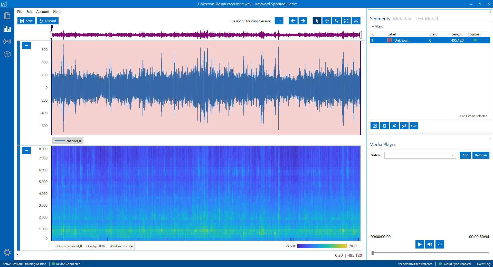
Displayed audio signal in the following figure belongs to a noisy restaurant. The entire range of the signal has been annotated with the “Unknown” label.
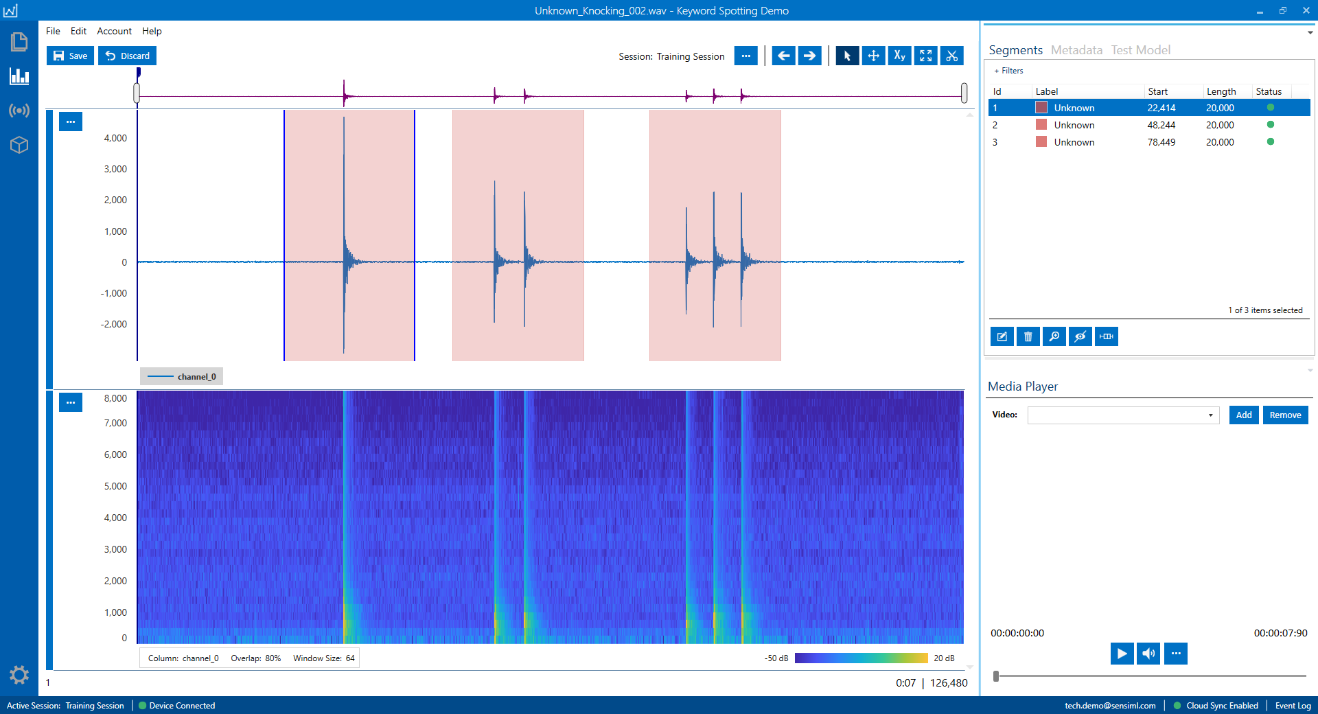
In addition to random noise, you need to have a set of random audio words in your Unknown dataset to reduce the chance of false positive detections. These audio events usually consist of words with variable lengths and different pronunciations. The content of these audio words should not be too similar to the project keywords or other audio signals that are already in the dataset. These types of Unknown signals are not limited to the human voice and can include very distinct intense audio events that may happen frequently in the deployment environment.
As an example, the following figure displays an audio signal made by knocking on a table. These events are labeled with the segments of the same default length as is used for the keywords.
Building a Keyword Spotting Model
We use the SensiML Analytics Studio to build our keyword spotting model. Login to your account and open your project.
Here are the steps you will take to create any model in Analytics Studio:
Prepare Data: In this step, you generate a query to specify what portion of your annotated data is taken to train the model.
Build Model: You setup the model generator pipeline to create and optimize your keyword spotting model. In this step, your annotated data is preprocessed and is used is training and cross validation tasks.
Explore Model: You evaluate the model performance based on the information provided by summary metrics and visualizations.
Test Model: You can run the generated classifier on a test dataset that has not yet been utilized for the training/validation process. As explained in the data annotation section, we use the “Set” metadata column to specify the test data. This dataset must have the same characteristics as the train/validation datasets such as ambient noise level, diversity of subjects. You can inspect the behavior of your classifier in Analytics Studio and the Data Studio.
Prepare Data
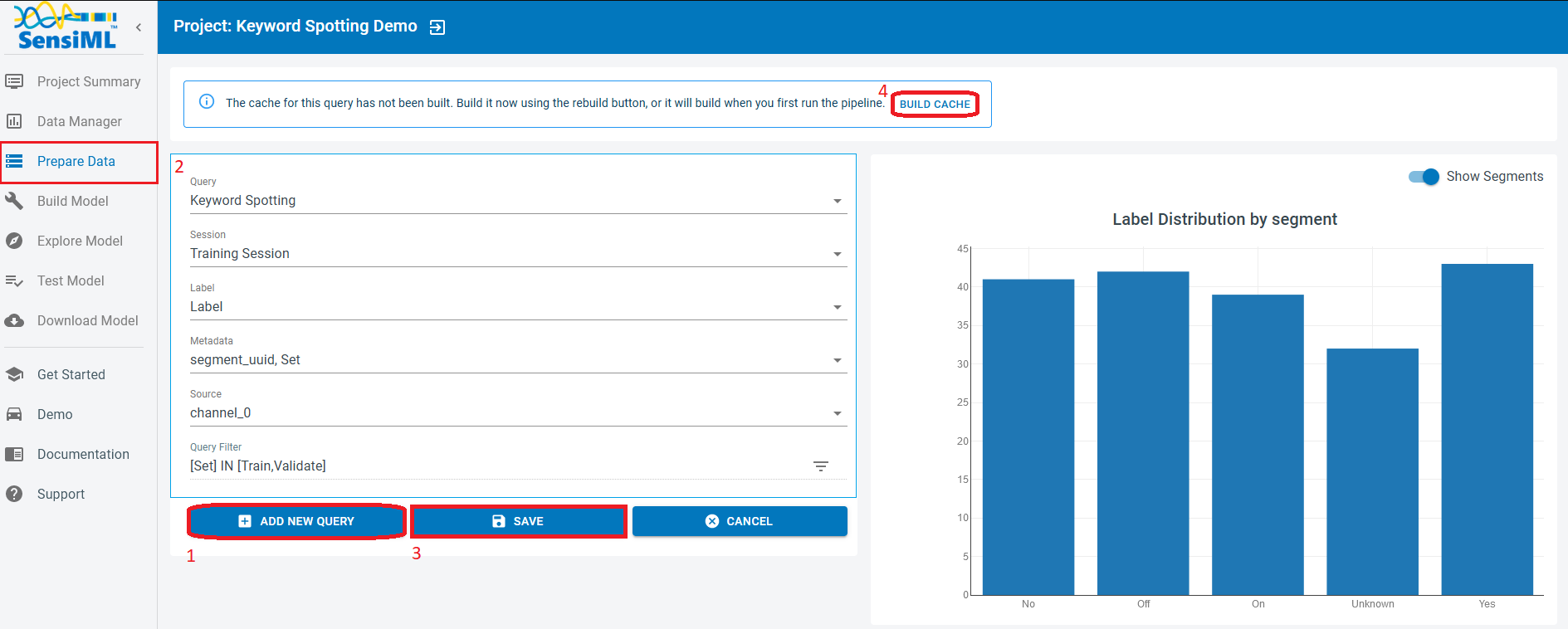
Click on the “Prepare Data” menu item from the left side of the Analytics Studio.
To create a new query
Click on the “Add New Query”
Fill in the query form to extract the appropriate data.
Query: Choose a name for your query.
Session: Select the session you used in the Data Studio to segment and annotate your capture files. Here, we use the labels stored in “Training Session”.
Label: Select the label group under which you annotated your data. Default is “Label”
Metadata: Choose all the metadata items you need to filter the data for your model. For example, if you are tracking the Training and Testing datasets in the “Set” column, you choose the column “Set” along with other metadata columns you need to slice the input data.
Source: “channel_0” is the name of the column that stores the audio data.
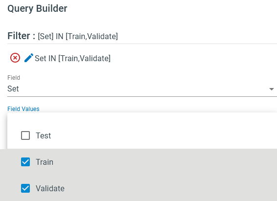
Query Filter: Click on the triangle-shape edit icon on the right and put your desired fields and criteria to filter out the data. For instance, we target column “Set” to extract “Train”, and “Validate” subsets.
Save the query and check out the segments size/label distributions.
When you save a query, you need to click on “Build Cache” in order to execute the query and to complete the data preparation for the pipeline.
Tip
Over the course of your project, if you add/remove recordings/labels and/or change the query conditions, you need to build the cache.
Note
We do not use the “Test” data in this query. This dataset is used independently to evaluate the model performance.
Model Builder Pipeline
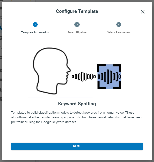
SensiML pipelines are designed to be modular and reusable. This allows users to quickly create and modify models to accommodate their needs. Any pipeline can be customized with different preprocessing, feature extraction, and machine leaning techniques to best fit the data and application. In this tutorial, we use the “Keyword Spotting” template to construct our pipeline.
Open the Build Model page
Select the Keyword Spotting template.
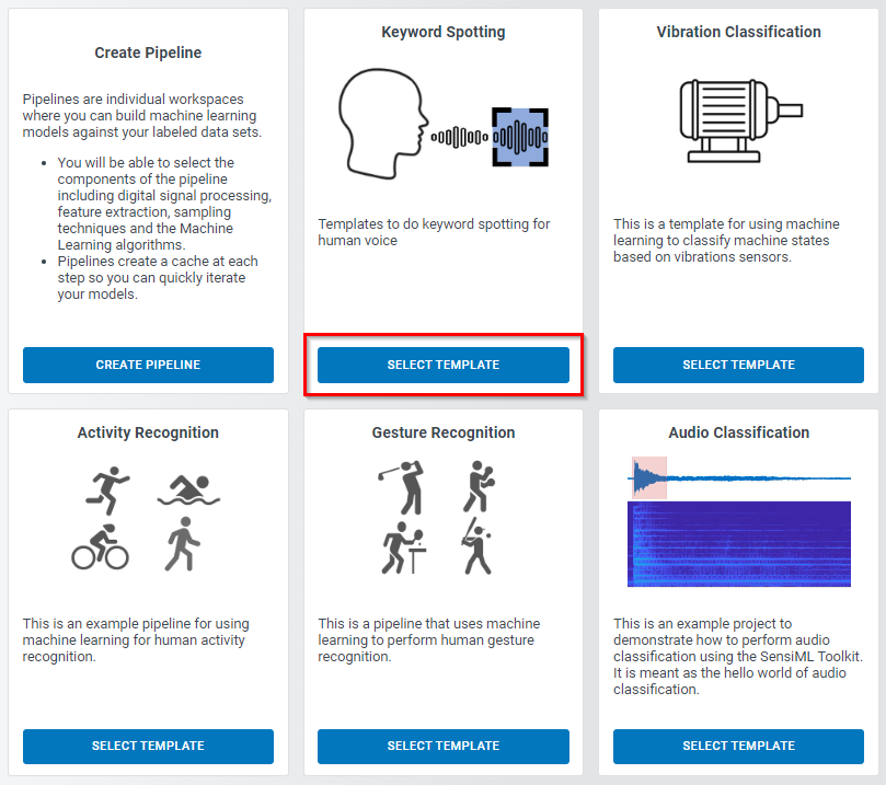
This template helps you to rapidly set up a pipeline that processes your data and trains your audio classification algorithm. Click on the “Next” button in the “Configure Template” box to go to pipeline selection step.
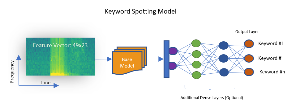
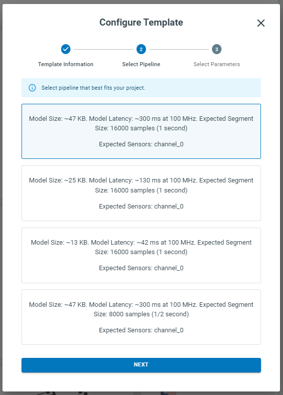
Select one of the listed pipelines based on your device capabilities and the offered model specifications. Please pay attention to the Expected Segment Size. which must be compatible with the size of your annotated segments and the keyword length. We recommend you first start with the smallest but fastest model (say second model in the following figure). For most applications with a few keywords and limited noise level, the smallest model usually achieves acceptable results. There is usually a trade-off between accuracy and latency. If the real-time response is more critical, then it might be necessary to compromise on accuracy to gain an acceptable latency. However, if accuracy is more important than latency, then it can be desirable to increase the model size and accept an increase in latency. It is also necessary to consider the available hardware resources, as larger models exhaust more computing power. In this tutorial, we use the 25 KB model (second in the following list). This model is a deep Convolutional Neural Network (CNN), with multiple rounds of depth-wise convolutions and max pooling, all implemented in TensorFlow framework.
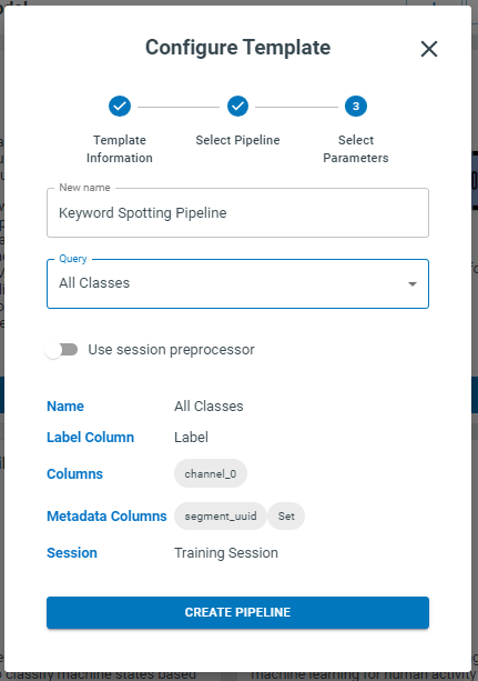
In the last step of template configuration, you choose a name for the pipeline and assign the name of the query you already created for data extraction. Click on “Create Pipeline” when you are done.
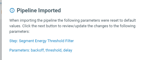
Once the pipeline is generated, there are a few parameters that might need to be adjusted depending on your application and the characteristics of the captured signals. Follow these steps and alter these parameters if needed. The following sections give you some idea on how to make proper adjustment.
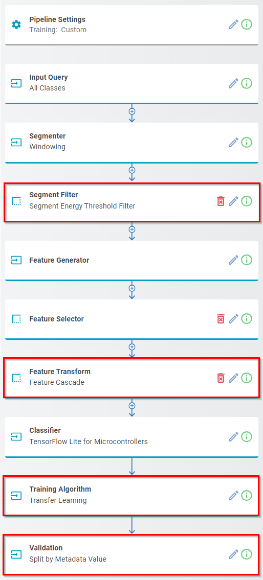
Pipeline Layout
You will notice all steps in the pipeline are automatically filled out from the Keyword Spotting Template we selected, but there are four steps we want to point out that can be useful for tweaking the parameters to be more customized for your dataset. Note - the keyword spotting template has already set these steps up with default values, the sections below give you more options for customizing the pipeline to work with your dataset if you are not getting good results
Segment Filter
Training Algorithm (Transfer Learning)
Validation
Feature Transform (Optional)
Note
The other pipeline steps have already been customized from the keyword spotting template that we selected earlier. Below you can find a brief description of what each step does.
Input Query: Holds the name of the query that is used to extract data to run this pipeline. This query picks all audio segments that fall into the “Train” and “Validate” categories.
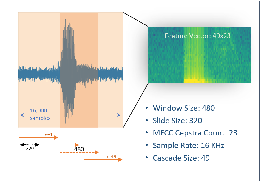
Segmenter [Windowing]: Defines how the annotated data is parsed into successive overlapping segments. Data series are chopped into sliding windows of 480 samples with the slide size of 320 samples.
Feature Generator [MFCC]: Uses Mel Frequency Cepstral Coefficients (MFCC) filter to extract significant characteristics of each data window in the frequency domain. In this model, we extract 23 features out of each set of 480 samples.
Feature Quantization [Min/Max Scale]: Maps the elements of the feature vectors to integer values between the specified minimum and maximum.
Feature Transform [Feature Cascade]: Combines 49 consecutive feature vectors, each holding 23 coefficients.
Classifier [TensorFlow Lite for Microcontrollers]: Specifies the machine leaning algorithm used to generate the model.
In the following sections, we will describe the highlighted pipeline blocks, and will explain how they can be customized to address some of the requirements.
1. Segment Filter
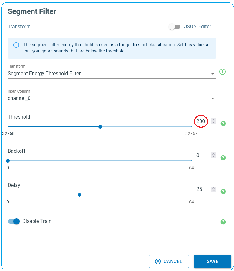
We set our Segment Filter step to Segment Energy Threshold Filter. The purpose of this is to avoid triggering the audio classification all the time, to optimize device power consumption. Moreover, most devices are unable to register the input data at the time of producing classifications and hence some parts of the acoustic signal are lost, potentially influencing the model performance. To partially address this issue, we trigger classifications based on the amplitude of the input audio within a given interval. In this example the audio data series is evaluated against the energy threshold condition, as it being ingested in packets of 480 samples. If the absolute amplitude of the signal is larger than the defined energy threshold, device starts the classification algorithm. In noisy environments, this method helps with energy conservation, and with minimizing the data loss owing to the successive adjacent classifications.
The following diagram displays a signal that contains five keywords and is captured in a noisy environment. We set the energy threshold at 200, well above the noise level to keep the model only sensitive to the interested audio events. This way our device does not spend its valuable energy resources to classify the noisy background.
Tip
The level of energy threshold depends on the microphone sensitivity and the environment condition. Please carefully adjust this threshold based on data collected in a realistic environment.
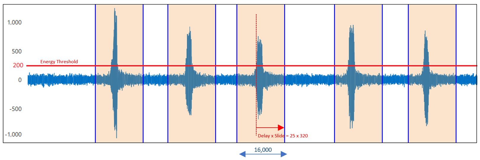
The parameters of the energy threshold filter are
Threshold: If the absolute value of the registered audio data is above the threshold, the classification is triggered. In the above diagram, the red horizontal line represents the threshold level.
Backoff: This parameter tells the device how many more classifications are required after the first one gets triggered by the threshold condition. For instance, Backoff=0 means that there are no additional classifications after each classification started due to the energy level of the signal. If backoff=1, one extra classification (two in total) is made per event. Classifications are spaced by slide value specified in the “Windowing” block of the pipeline (i.e. 320 sample).
Delay: It is the factor that determines how long the model should postpone the classification process after the threshold condition is satisfied. Our model processes the data live as it is streamed, and the threshold condition is checked in every registered 480 samples (30 microseconds). Most often the audible events like speech keywords are longer and therefore device needs to wait for a while to register the whole event before it produces the classification. Note that this model requires 1 second of data to produce classification. The classified region is divided to 49 successive windows of size 480 that are 320 samples apart. Therefore, this model is potentially capable of production classifications at every 320 samples. To avoid the latency issue, it is preferred to generate only one classification for each event but leaving enough time for the event of interest to be registered by the device. So, choose a delay factor wisely, a value that is more compatible with the keyword patterns in your project. Setting Delay to 25 for the cascade size of 49 puts the center of the event on the center of the classification window. Larger values force the center of the event shift toward the beginning of the classification window.
Doing the math
To be exact, the covered range of each segment will be 15,840 samples, 320*(49-1) + 480. In this document, for the sake of simplicity we use 16,000 for the length of the classified regions.
Tip
The energy threshold filter is useful when the model is flashed to the device and works in real time. Turn on “Disable Train” to deactivate this function during the training process and to use the data augmentation benefits of the sliding data segments.
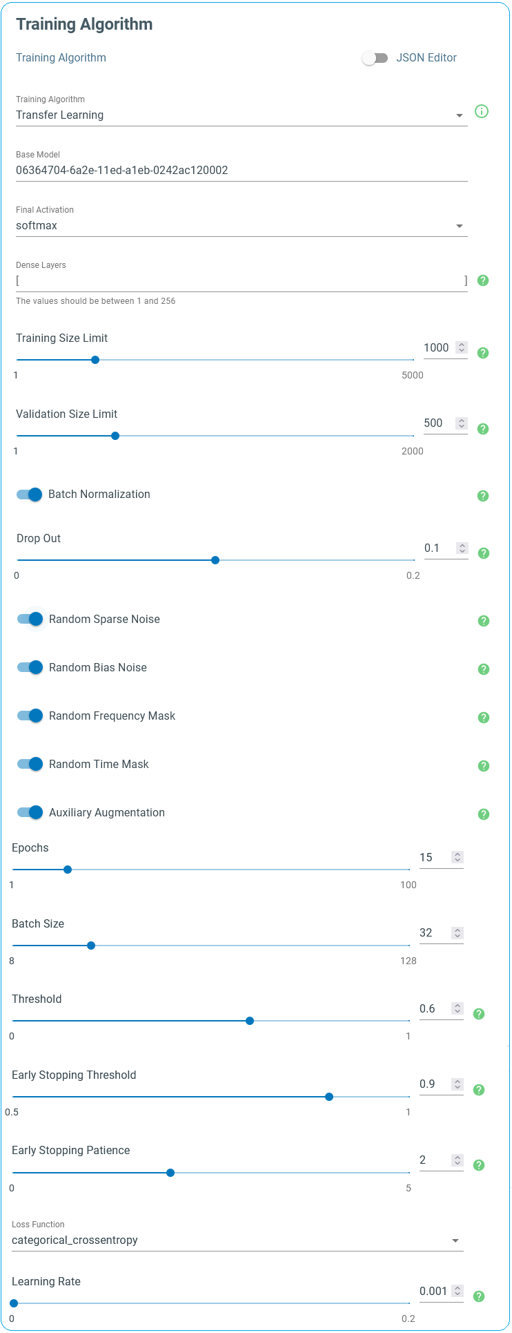
2. Training Algorithm
We set our Training Algorithm step to Transfer Learning. Transfer Learning is a machine learning technique that involves the transfer of knowledge from an original model to a target model. This is done by reusing the base model’s parameters, weights, and network architecture as a starting point the training process of the target model. The goal of transfer learning is to reduce the amount of training time and data required to build model without compromising its accuracy. Transfer learning is a popular method for training deep learning models and is especially useful for tasks where a large dataset is not accessible or hard to obtain.
The SensiML keyword spotting model starts from a convolutional neural network that has been already trained using a large dataset. In this project, the weights of the CNN have been already optimized using the Google speech command dataset. During the transfer learning process, the weights of the base model are evolved using the training data specifically collected for the target application. The transfer learning only trains the output layer and any extra dense layers before that. During the training process, the convolutional core of the base model remains intact.
Here is the list of the important parameters one can change to control the training flow.
Dense Layers: A list of additional dense layers to add more complexity to the model to improve the model performance, especially when the project includes a large number of keywords or words that have close pronunciations.
Training/Validation size limit: In the beginning of each training epoch, the training sample is resampled to form a uniform distribution across all keywords and the unknown events. To avoid having very long training time for large datasets, these parameters control the maximum number of randomly selected samples per label in each training epoch.
Batch Normalization: Batch normalization works by normalizing the inputs of each layer with the mean and variance of the batch. Batch normalization increases the stability of the network and reduces the risk of overfitting, and it enables using larger training rates, resulting in faster training.
Drop Out: It is a type of regularization technique used in deep learning. When activated, the specified fraction of the layer outputs is randomly dropped out (they are set to zero) during training. This has the effect of making the model more robust and less prone to overfitting.
Note
Some of the parameters, such as “Training Algorithm”, “Base Model” and “Final Activation” ought to remained unchanged.
“Batch Normalization” and “Drop Out” are only effective in the presence of the additional dense layers and they act on the outputs of each layer.
Data Augmentation Techniques: Introduced by either altering the 2-dimentional feature vector (here it is 49x23) or adding feature vectors from a similar project. Feature vectors have two axes, time frequency. Activating these
Random Sparse Noise: Alters a fraction of the feature elements.
Random Bias Noise: Applying random bis noise to the feature vector.
Random Frequency Mask: Randomly replaces a fraction of rows (along the time axis) with a constant value.
Random Time Mask: Performs a similar action but along the columns (frequency axis).
Auxiliary Augmentation: Adds additional feature vectors of background noise for keyword spotting models. This helps when a project lacks a comprehensive dataset of Unknown ambient noise.
Epochs: Maximum number of training iterations
Batch Size: During each training epoch, dataset is randomly divided into small batches. Batch size is used to determine the size of the data set that will be passed through the neural network when training.
Threshold: The model outputs the classification in the form of probabilities. If the classification probability is less than the specified threshold, the model output will be uncertain and hence it returns “Unknown” instead.
Early Stopping Threshold: During the training process, the model accuracy is monitored using the validation set. If the accuracy is larger than the specified early stopping threshold is a number of successive epochs, the training process is automatically terminated to avoid overfitting. If the early stopping criteria is not satisfied, all training epochs are exhausted and then the final model is returned.
Early Stopping Patience: The number of successive epochs that should meet the early stopping condition to stop training.
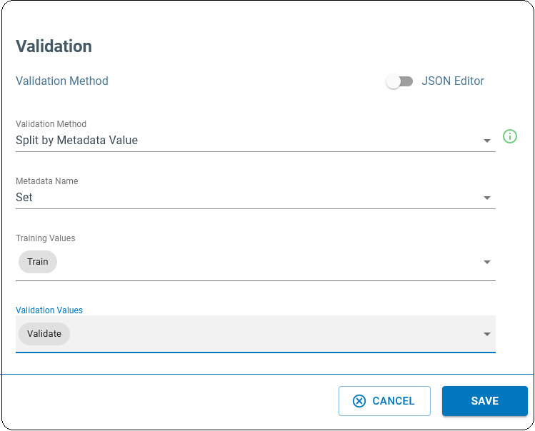
3. Validation
We set our Validation step to Split by Metadata Value. This uses a subset of our labeled data to assess the performance of the trained model. Validation is the method to evaluate how well a model can make predictions on unseen data. Validation helps to identify any problems with the model, such as overfitting or bias, and to determine which parameters are most effective for the given problem. In this project, we have collected the validation dataset separately. Go to the validation block of the pipeline and choose the “Split by Metadata Value” method and set other parameters accordingly.
The training algorithm uses the validation set to monitor the training progress and it potentially stops the process to avoid overfitting whenever the desired accuracy is achieved. For this purpose, we use the fraction of data whose “Set” column is set to “Validate”. Please keep in mind that just the “Train” subset is used for the training job.
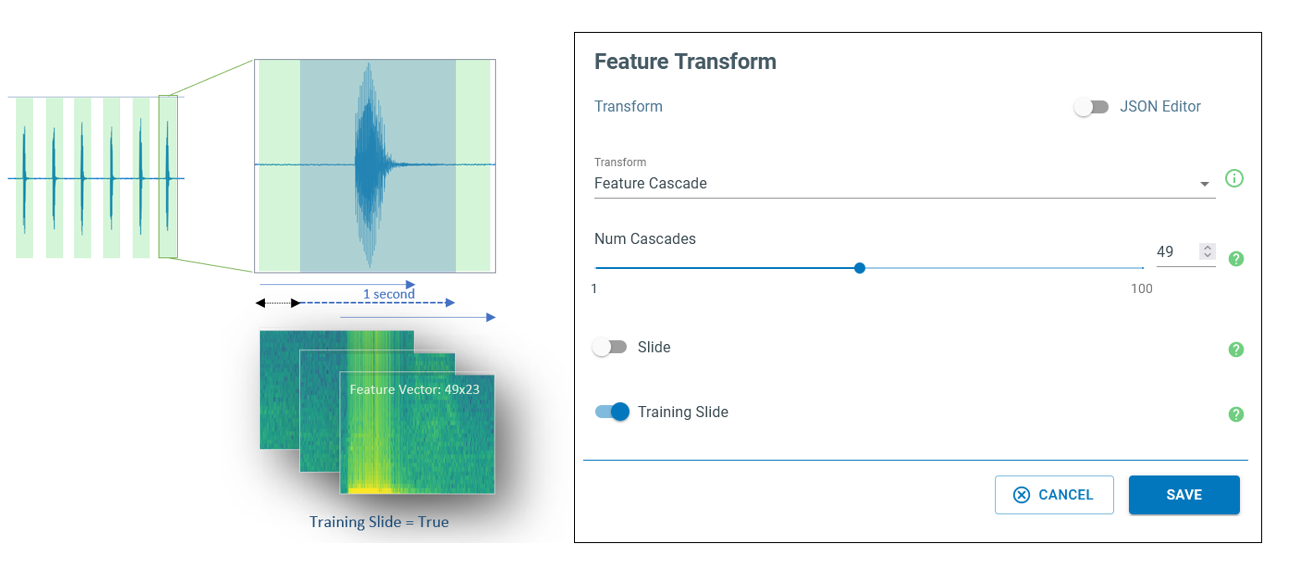
4. Feature Transform
We set our Feature Transform step to Feature Cascade. As mentioned earlier, for each window of 480 samples 23 MFCCs are generated. Each annotated segment is spanned by these windows that are separated by 320 samples. Therefore, to cover 1 second of data (at the rate of 16 kHz), feature vectors of 49 adjacent windows are stacked. If a labelled region is larger than 1 second, this process generates more than one 49x23 features. This can help when the collected data is limited and is used as a means of data augmentation.
Go to the Feature Transform block of your pipeline that is already loaded by the Feature Cascade function.
Num Cascade: This is a characteristic that depends on the base model and therefore should not be changed at this point.
Slide: If activated, performs the sliding process when generating the classification on the device. The model inference flow is controlled by the “Energy Threshold Filter” parameters if available.
Training Slide: If activated, the sliding action can potentially produce more than one feature vector for a labeled segment, that can be leveraged to mitigate the small size of collected data to some extent.
Model Optimization
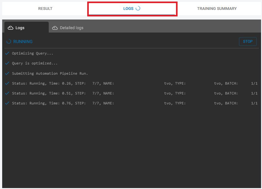
Once you are happy with the pipeline, click the Run Pipeline button to start the training process. Training time depends on the size of your dataset and the number of training epoch needed to be passed.
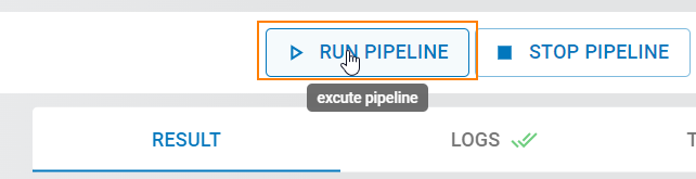
You can monitor the progress of the pipeline in the “Logs” tab.
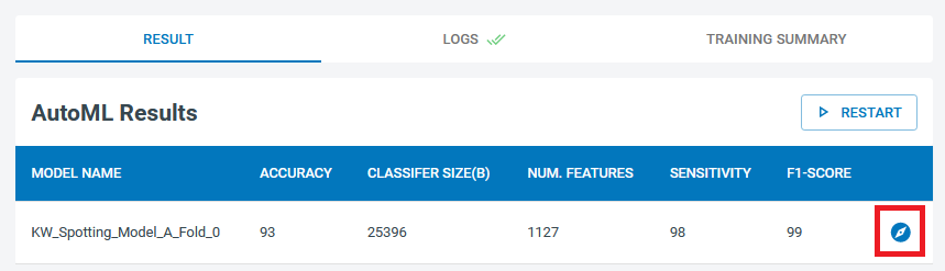
At the end of the optimization process, the accuracy of the model together with other metrics are listed in the results table. For further assessments, you can click on the “Explore Icon” (denoted by the red box in the next figure).
If the model accuracy is extremely poor, explore its training metrics and try out some of the remedies explained in the following section.
Due to the random nature of the training algorithm, repeating the optimization task without changing the pipeline parameters might return different results. So if you get bad results, try re-running the pipeline before making any conclusions and updating the pipeline parameters.
Explore Model
In Analytics Studio, go to the “Explore Model” from the left menu item. This page presents a summary of the training/validation process and the efficiency of the model in making correct predictions.
Select “Confusion Matrix” from the top menu bar. A confusion matrix is a table used to describe the performance of a classification model on different subsets of data for which the true values are known. It allows visualization of the performance of an algorithm. Each row of the matrix represents instances in the actual class while each column represents instances in the predicted class. A confusion matrix makes it easier to see where a model makes misclassifications and offers valuable information to take further actions to improve the model. For instance, if there is a bias towards a single class by providing a very unbalanced dataset, the confusion matrix reveals many misclassifications in favor of that class.
In addition to the keywords and the “Unknown” label, you see an extra column in these tables labeled as “UNK”. This class is reserved for those instances with uncertain predictions, where the classification probability is less than the “Threshold” value in the Transfer Learning block.
Ideally, reasonable models exhibit high accuracies and low false positive rates for all classes. Their training and validation confusion metrices look similar in terms accuracy, sensitivity, and false/true positive rates. Any significant differences could be taken as a clue for over/under-fitting.

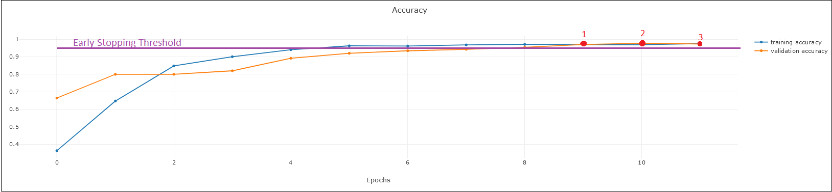
Another way to study a neural network is to monitor how its different evaluation metrics rise and fall over successive epochs. The accuracy of a classifier is one of the most critical parameters to consider as the training process advances. In general, the accuracy of the model on the training dataset is improved with the epoch number (blue curve in the following diagram). However, the validation accuracy (orange curve) might not progress as expected. In ideal cases, training and validation accuracies relatively reach to the same level in the end.
In the example below, early stopping threshold is set at 0.95 (purple horizontal line) with patience of three (red symbols), meaning that the validation accuracy must be better than 0.95 in three successive epochs for training to be stopped.
A model is over-trained if the training accuracy improves while the validation accuracy is not getting any better or it is degrading. In this case, you should consider lowering the early stopping threshold, revisiting the early stopping patience, or the number of epochs.
If the training accuracy has been flattened out at its maximum, but the validation accuracy is zig-zagging (randomly jumping up and down) or has not reached the same level, here are the options that could potentially resolve the issue:
Consider Lowering the learning rate while increasing the number of training epochs to allow the neural network weights to evolve slower.
Consider increasing the number of training epochs if the model accuracy monotonically increases with training epochs but does not reach the desired early stopping threshold.
Consider collecting more data in a different audio environment.
Reconsider the model architecture. Sometimes the model architecture itself may be the problem. Consider using and/or altering dense layers or trying a template of different complexity.
Use larger data size at each training epoch. You can simply do this by increasing the maximum training size.
Revisit your data augmentation strategy.
Test Model
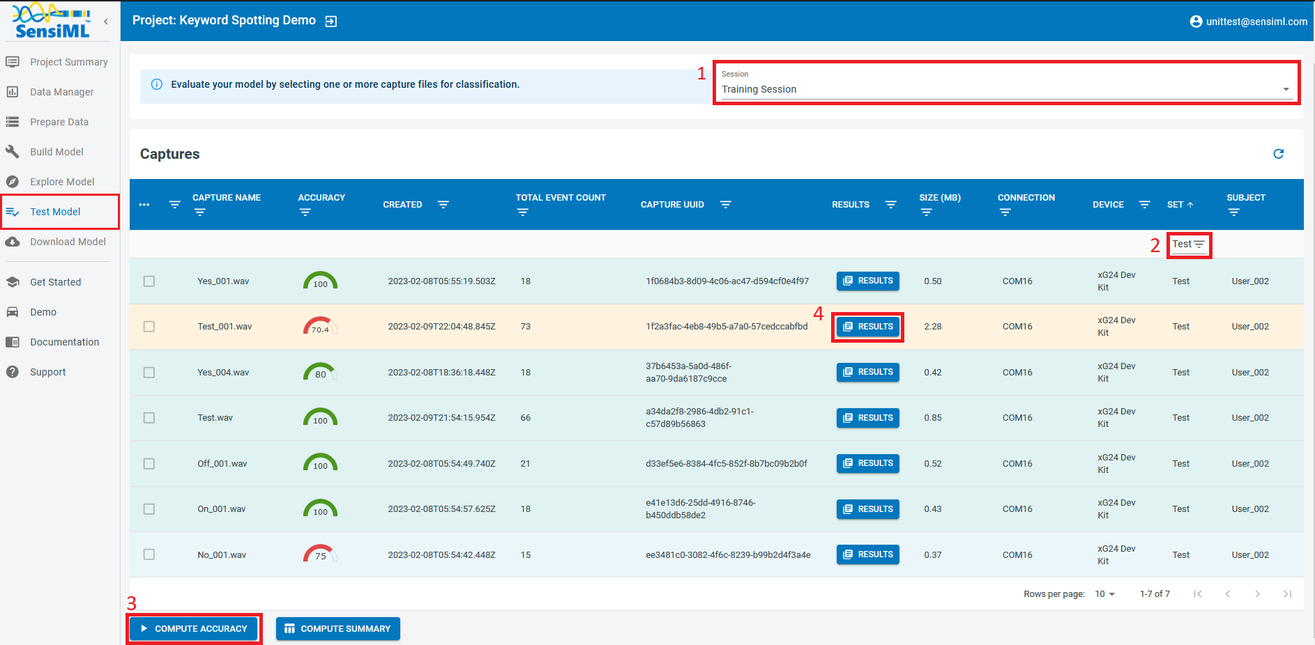
You can set the performance of your model in Analytics Studio by visiting the “Test Model” page and choosing a model from the list.
Choose the annotation session that stores the ground truth labels.
From the “Set” metadata column, choose the “Test” dataset. Note that this data has already been seen by the model during training and validation.
Select the desired capture files for testing purposes and click on “Compute Accuracy.”
Click on the “Results” button to see the classification results as it is visualized in the bottom of the page.
Testing a Model in the Data Studio
The Data Studio can run models in real-time with your data collection firmware or it can run them on any CSV or WAV file that you have saved to your project in the Project Explorer.
Running a Model on Files in the Project Explorer
Open the Project Explorer in the left navigation bar.
Select the files you want to run with the model and Right + Click > Run Model.
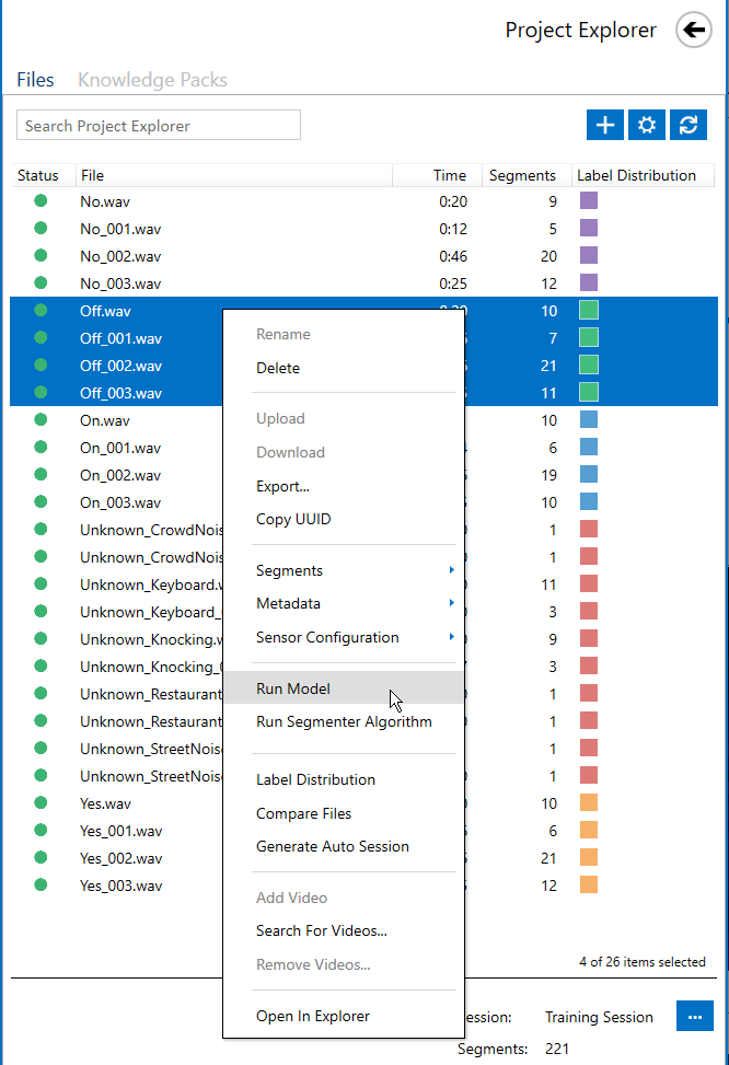
Select the model and save the classification results. Note: Save your results in a different session than your training/ground truth session
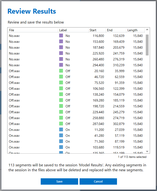
You can now open the files you selected to view the classification results of the model.
Running a Model in Real-Time
Click on the Test Model button in the left navigation bar.
Select a device that is running data collection firmware.
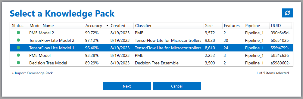
Select a Knowledge Pack.
As your device collects audio data, the Data Studio will graph the sensor data and model classifications in real-time.
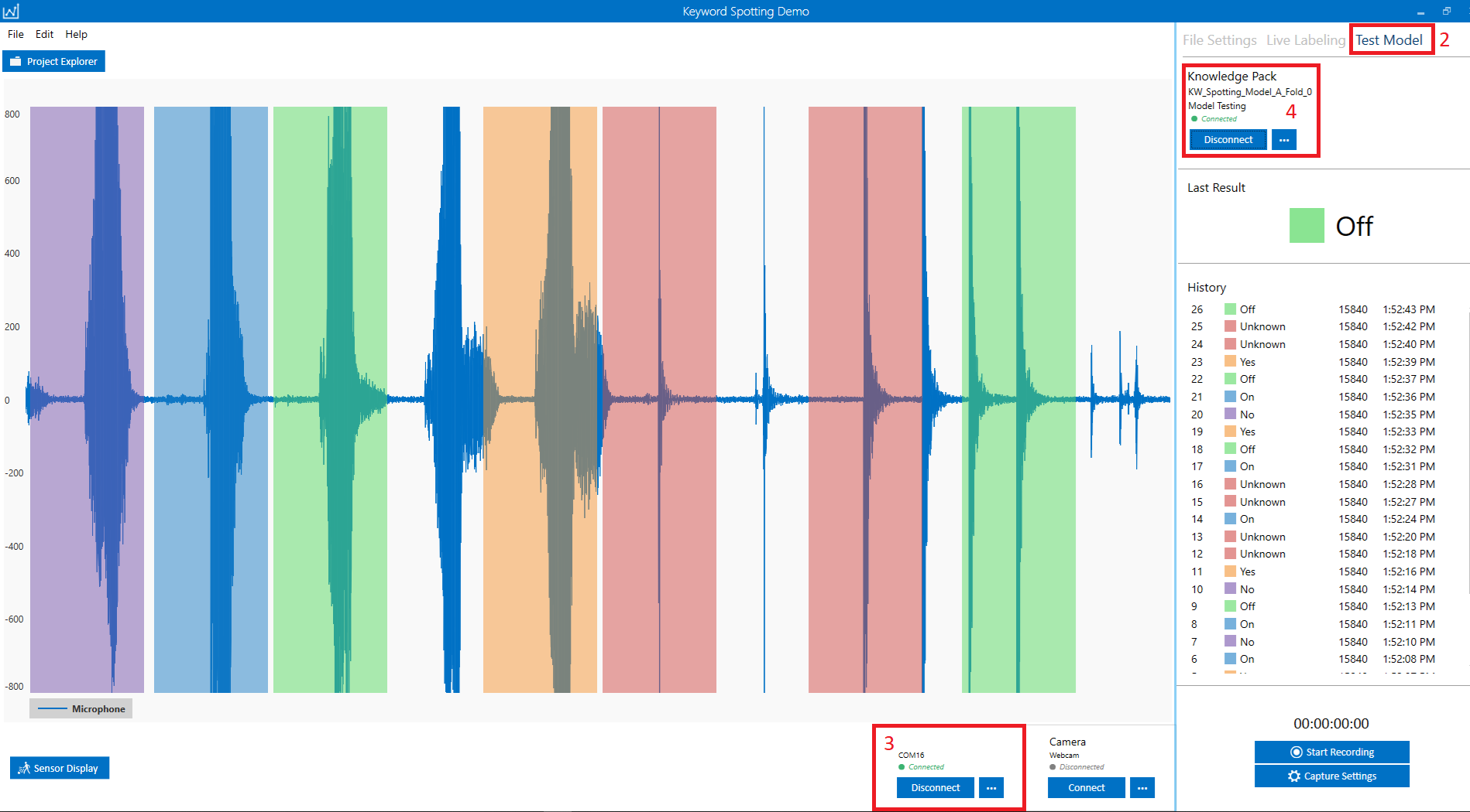
You can also click the Start Recording button and save your captured data and the model results.
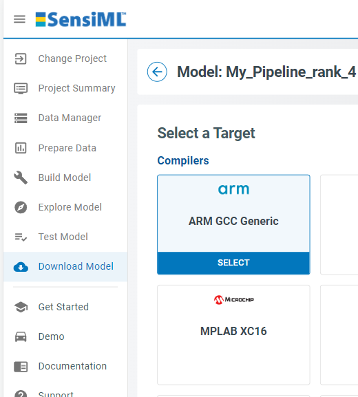
Deploying a Model to a Device
In order to deploy your model, you need to download it in the form of a Knowledge Pack. Please refer to the Generating a Knowledge Pack Documentation for further details.
To flash your knowledge pack to your embedded device, follow the Flashing a Knowledge Pack Documentation.
To see classification results, you may use a terminal emulator such as Tera Term or the Open Gateway.
For additional documentation please refer to the Running a Model on Your Embedded Device Documentation.