Boxing Punch Activity Recognition

Overview
In this tutorial, we are going to build a boxing punch activity recognition application that can run entirely on a Cortex-M4 microcontroller using SensiML Analytics Toolkit and TensorFlow Lite for Microcontrollers. The model we create will use the onboard IMU sensor as input, SensiML Knowledge Pack for feature extraction, and TensorFlow Lite for Microcontrollers to perform classification.
Objectives
Demonstrate how to collect and annotate a high-quality dataset of boxing punch motions using the SensiML Data Studio
Build a data pipeline to extract features in real-time on your target device.
Train a neural network using TensorFlow to classify the extracted features.
Quantize the trained neural network and load it into the SensiML pipeline.
Convert the pipeline into a Knowledge Pack and flash it to our target embedded device.
Perform live validation of the model running on-device using the SensiML TestApp
Collecting and Labeling Sensor Data
For every machine learning project, the quality of the final product depends on the quality of your curated data set. Time series sensor data, unlike image and audio, are often unique to the application as the combination of sensor placement, sensor type, and event type greatly affects the type of data created. Because of this, you will be unlikely to have a relevant dataset already available, meaning you will need to collect and annotate your own dataset.
To help you to build a data set for your application we have created the SensiML Data Studio, which we are going to use for collecting and annotating our corpus of Boxing punch motions. The dataset for this tutorial can be downloaded from this link:
Unzip the files and import the dataset to the Data Studio by clicking
Import Project
Below you can see a quick demonstration of how the Data Capture lab enabled us to create an annotated boxing punch activity data set. In the next few sections, we are going to walk through how we used the Data Studio to collect and label this dataset.
Determining Events of Interest
Detecting and classifying events is ultimately the main goal of a time series application. In general, events fall into one of two types: continuous or discrete.
Continuous “Status” Events
Continuous events are events that happen over longer, gradual intervals or periods of time. Think of them like you are looking for the current status of the device. An example of this includes a motor fault detection sensor. In this example, the sensor will detect a continuous “Normal” status or in a continuous “Failure” status. In a fitness wearable, you may be looking for the user’s activity status (Running, Walking, Resting).
Discrete “Trigger” Events
Discrete events are events that have discrete trigger actions that the application needs to be trained for. In this boxing wearable example, the sensor will detect the trigger events of “Uppercut” or “Jab”. But ignore all other input. You may find that detecting discrete events is a more challenging problem than continuous events. This is because of all the different types of actions a user may do with your device that are do not fall within “Uppercut” or “Jab”. Therefore, collecting enough data to prevent False Positives is critical.
Why is this important?
The type of event you are trying to detect will change the way you want to train your raw sensor data in the SensiML toolkit. In the SensiML Data Studio, you can put what we call Segment Labels on any portion of your sensor data. This allows you to accurately mark wherein the dataset each type of event is occurring.
Capturing Environmental Context
In addition to labels, it is also important to capture information about the environment. Capturing this contextual information enables you to build highly tailored models. Additionally, it makes it possible to diagnose why a model might be failing for subsets of your data.
For example, in this boxing activity dataset, we captured several contextual properties such as subject size, boxing experience, dominant hand, etc. Using these we would be able to build a model for novice boxers and expert boxers that most likely would be more accurate and compact than attempting to build a single general model.
You can capture the contextual information in the Data Studio using the metadata properties. Metadata are applied to the entire captured file, so when you are creating your data collection strategy think carefully about what you information you may need. Metadata can be created as a selectable dropdown or manual entry allowing flexibility for your data collectors.
The video below goes into how to create and update metadata and segment label properties in the SensiML Data Studio.
Capturing Data
Now that we have set up our project, it’s time to start collecting data. To collect data, we will go to the Capture mode in the Data Studio. The first thing we need to do is to set up the sensor that we would like to use. For this tutorial, we are using the Chilkat. There are several other sensors with built-in support. You can also add your sensors and boards by following the instructions in the Simple Streaming Interface Documentation.
We will configure this sensor to capture both IMU and Gyroscope data at a sample rate of 104Hz. In this tutorial we are streaming the data over BLE, however for higher sample rates we typically either store the data directly to an internal SD card or stream it out over a serial connection. We have examples in our SDK for both which you can follow to implement on your device.
After specifying our sensor configuration, we will connect to the device and be ready to record live data. We will use our laptops camera to record video, which we will sync up later.
The captured data will be saved locally and synced up to the SensiML Cloud. This allows other members of your team who have permission to see and label your new captured file. Alternatively, If you already have a data collection method for your device, the Data Studio can import CSV and WAV files directly so you can still use it for annotating the data.
The video below walks through creating a sensor configuration, capturing data, and syncing the data to your cloud project.
Annotating Events of Interest
The Data Capture lab has a manual label mode and an automatic event detection mode. For this tutorial, we are going to use automatic event detection. Automatic event detection using parameterized segmentation algorithms which are parameterized based on the events and dataset you provide. We have selected the windowing threshold segmentation algorithm and already optimized the parameters based on the dataset collected so far.
To perform automatic event detection on a new capture, select the capture and click on the detect events button. The SensiML Cloud will process the file and return the segments it finds based on the selected capture. Event detection only detects that an event has occurred, it does not determine what type of event has occurred. After the Data Studio detects the events, you will then need to apply a label to them. To label a segment, click the edit button and select a label that is associated with that event.
The video below walks through how to label the events of a captured file in the SensiML Data Studio.
Building a Query
The SensiML Analytics Studio is where you can create queries to pull data into your model, build models using AutoML, validate model accuracy against raw signal data and finally download your model as firmware code for the target device.
For the next part of the tutorial, you’ll need to log into Analytics Studio where we will create the query against our model.
Creating a Model to Classify Boxing Punches
At this point in the tutorial, we will use Google Colab to train a neural network with TensorFlow. You can also use your local environment if you have TensorFlow installed. Click here to get the notebook and try yourself.
The video below will walk through training a TensorFlow model in Google Colab.
SensiML Python SDK
We are going to connect to SensiML’s cloud engine using the SensiML Python SDK. If you have not yet created an account on SensiML you will need to do that before continuing. You can create a free account by going here
To install the client in the Google Colab environment run the command in the following cell.
!pip install sensiml -U
Next, import the SensiML Python SDK and use it to connect to SensiML Cloud. Run the following cell, which will ask you for your username and password. After connecting, you will be able to use the SensiML Python SDK to manage the data in your project, create queries, build and test models as well as download firmware. Further documentation for using the SensiML Python SDK can be found here
from sensiml import SensiML
client = SensiML()
Next we are going to connect to our Boxing Glove Gestures Demo Project. Run the following cell to connect to the project.
client.project = 'Boxing Glove Gestures Demo'
Creating a Pipeline
Pipelines are a key component of the SensiML workflow. Pipelines store the preprocessing, feature extraction, and model building steps. When training a model, these steps are executed on the SensiML server. Once the model has been trained, the pipeline is converted to a firmware code that will run on your target embedded device. For more documentation on pipelines see the advanced model building tutorial. To create a new empty pipeline, run the cell below.
client.pipeline = 'TensorFlow Lite Micro'
Sandbox TensorFlow Lite Micro does not exist, creating a new sandbox.
Now we are going to add our preprocessing steps to the pipeline, for a detailed description of the features available in a pipeline see the documentation here.
You can also list the functions by running client.list_functions(qgrid=False) in a code cell of the notebook.
Adding Steps to the Pipeline
The pipeline for this tutorial will consist of the following steps:
The Input Query which specifies what data is being fed into the model
The Feature Generators which specify which features should be extracted from the raw time-series data
The Feature Transform which specifies how to transform the features after extraction. In this case, it is to scale them to 1 byte each
The Feature Selector which selects the best features. In this case, we are using the custom feature selector to downsample the data.
The code in the following cell sets our initial variables, then specifies each step in the pipeline. For now, you don’t need to dig into each of these steps, but just know that the end result will be a feature vector scaled to 1-byte values for each of the segments that were labeled in the Data Studio. We will use these features as input to our TensorFlow model.
sensor_columns= list(client.project.columns())+["Magnitude_ST_0000"]

client.pipeline.reset()
client.pipeline.set_input_query("GesturePunches") # specify the input data set to use
client.pipeline.add_feature_generator(            # Add Feature Generators
    [
        {'subtype_call': 'Statistical'},
        {'subtype_call': 'Shape'},
        {'subtype_call': 'Column Fusion'},
        {'subtype_call': 'Area'},
        {'subtype_call': 'Rate of Change'},
    ],
    function_defaults={'columns': sensor_columns},
)

client.pipeline.add_feature_selector([{'name':'Tree-based Selection', 'params':{"number_of_features":16}},])

client.pipeline.add_transform("Min Max Scale")     # Scale the features to 1-byte

client.pipeline.describe()
Generating Feature Vectors
At this point the pipeline has not been executed yet, we are just assembling the steps. To run the pipeline, execute the following cell. This will execute the pipeline on SensiML Cloud and return the results as a pandas DataFrame.
Once the pipeline is finished running, the results will be stored in the variable fv_t. A summary of the execution is stored in the s_t variable.
fv_t, s_t = client.pipeline.execute()
Executing Pipeline with Steps:

------------------------------------------------------------------------
 0.     Name: GesturePunches                        Type: query
------------------------------------------------------------------------
------------------------------------------------------------------------
 1.     Name: Magnitude                             Type: transform
------------------------------------------------------------------------
------------------------------------------------------------------------
 2.     Name: generator_set                         Type: generatorset
------------------------------------------------------------------------
------------------------------------------------------------------------
 3.     Name: selector_set                          Type: selectorset
------------------------------------------------------------------------
------------------------------------------------------------------------
 4.     Name: Min Max Scale                         Type: transform
------------------------------------------------------------------------
------------------------------------------------------------------------


Results Retrieved... Execution Time: 0 min. 0 sec.
fv_t.head()
| gen_0005_AccelerometerYMean | gen_0006_AccelerometerZMean | gen_0039_AccelerometerXLinearRegressionStdErr_0003 | gen_0046_AccelerometerXStd | gen_0067_AccelerometerXIQR | gen_0074_AccelerometerX25Percentile | gen_0082_AccelerometerY75Percentile | gen_0083_AccelerometerZ75Percentile | gen_0096_AccelerometerYminimum | gen_0110_AccelerometerYSum | gen_0130_AccelerometerXVariance | gen_0285_AXAY_cross_min_max_diff | gen_0306_AXAY_cross_mean_diff | gen_0309_AYAZ_cross_mean_diff | gen_0337_AccelerometerYTotArea | gen_0358_AccelerometerYAbsAreaDc | Punch | SegmentID | Type | segment_uuid | |
|---|---|---|---|---|---|---|---|---|---|---|---|---|---|---|---|---|---|---|---|---|
| 0 | 84 | 148 | 171 | 168 | 21 | 245 | 75 | 136 | 0 | 84 | 118 | 102 | 197 | 66 | 84 | 33 | Cross | 60 | Train | 6d5c5130-97f1-457b-8d9c-8ba2184fca2a |
| 1 | 90 | 149 | 184 | 181 | 72 | 204 | 78 | 157 | 0 | 90 | 135 | 102 | 190 | 69 | 90 | 32 | Cross | 61 | Train | e5de78f0-3ec1-40f1-bfaf-a5500c8dc86c |
| 2 | 101 | 151 | 162 | 160 | 93 | 181 | 93 | 151 | 0 | 101 | 108 | 102 | 183 | 74 | 101 | 31 | Cross | 62 | Train | e45bd9d8-f65f-41ff-8194-45b19eb9438e |
| 3 | 88 | 166 | 148 | 145 | 81 | 191 | 79 | 169 | 0 | 88 | 90 | 254 | 197 | 55 | 88 | 27 | Cross | 63 | Train | 1011ddf4-96fb-451f-b855-07d11da46572 |
| 4 | 80 | 174 | 152 | 149 | 71 | 195 | 85 | 169 | 0 | 80 | 95 | 254 | 200 | 44 | 80 | 49 | Cross | 64 | Train | 5c39ff84-75df-4508-ac64-99a198ea7e4d |
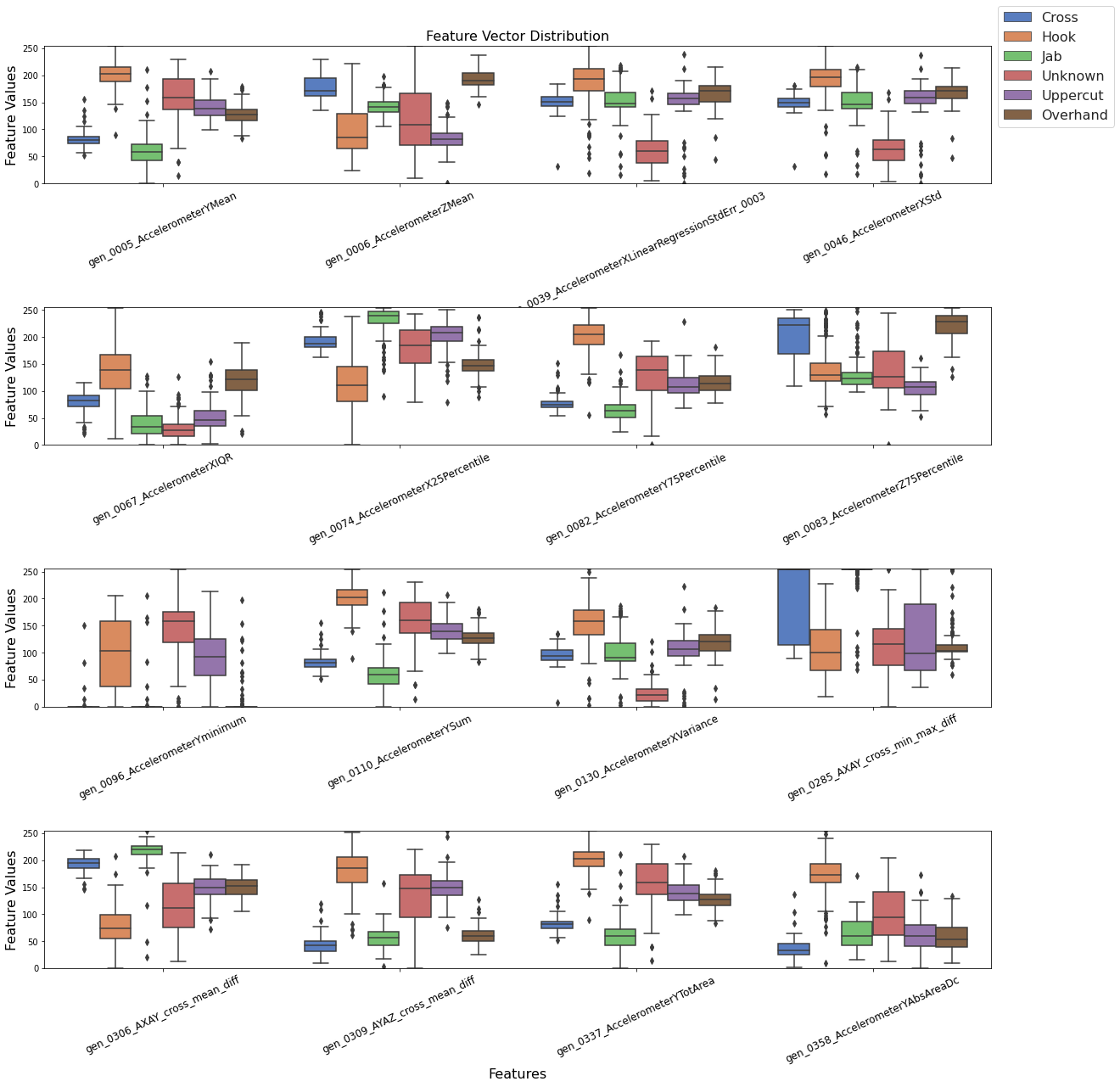
Run the following cell to see the distribution of feature each across the different classes. The best features will have low variance and good class separation.
client.pipeline.visualize_features(fv_t)
Now we have our features for this model, we will go ahead and train a TensorFlow Model in the Colab environment. We will start by splitting our dataset into train and validate groups. Our test set is not included in the query and will be used later.
The SensiML Python SDK has a built-in function for performing this split. You can also pass in the validation data test sizes. By default, they are set to 10% each.
x_train, x_test, x_validate, y_train, y_test, y_validate, class_map = \
    client.pipeline.features_to_tensor(fv_t, test=0.0, validate=.1)
-----  Summary  -----
Class Map: {'Cross': 0, 'Hook': 1, 'Jab': 2, 'Unknown': 3, 'Uppercut': 4, 'Overhand': 5}
Train:
 total:  645
 by class: [ 92. 120. 130.  91. 108. 104.]
Validate:
 total:  72
 by class: [ 8. 15. 11. 19. 11.  8.]
Train:
 total:  0
 by class: [0. 0. 0. 0. 0. 0.]
Creating a TensorFlow Model
The Next step is to define what our TensorFlow model looks like. For this tutorial, we are going to use the TensorFlow Keras API to create the NN. When you are building a model to deploy on a microcontroller, it is important to remember that all functions of TensorFlow are not suitable for a microcontroller. Additionally, only a subset of TensorFlow functions is available as part of TensorFlow Lite Micro. For a full list of available functions see the all_ops_resolver.cc.
For this tutorial, we will create a deep fully connected network to efficiently classify the boxing punch movements. Our aim is to limit the number and size of every layer in the model to only those necessary to get our desired accuracy. Often you will find that you need to make a trade-off between latency/memory usage and accuracy in order to get a model that will work well on your microcontroller.
from tensorflow.keras import layers
import tensorflow as tf

tf_model = tf.keras.Sequential()

tf_model.add(layers.Dense(12, activation='relu',kernel_regularizer='l1', input_shape=(x_train.shape[1],)))
tf_model.add(layers.Dropout(0.1))
tf_model.add(layers.Dense(8, activation='relu', input_shape=(x_train.shape[1],)))
tf_model.add(layers.Dropout(0.1))
tf_model.add(layers.Dense(y_train.shape[1], activation='softmax'))

# Compile the model using a standard optimizer and loss function for regression
tf_model.compile(optimizer='adam', loss='categorical_crossentropy', metrics=['accuracy'])

tf_model.summary()
train_history = {'loss':[], 'val_loss':[], 'accuracy':[], 'val_accuracy':[]}
Model: "sequential"
_________________________________________________________________
Layer (type)                 Output Shape              Param #
=================================================================
dense (Dense)                (None, 12)                204
_________________________________________________________________
dropout (Dropout)            (None, 12)                0
_________________________________________________________________
dense_1 (Dense)              (None, 8)                 104
_________________________________________________________________
dropout_1 (Dropout)          (None, 8)                 0
_________________________________________________________________
dense_2 (Dense)              (None, 6)                 54
=================================================================
Total params: 362
Trainable params: 362
Non-trainable params: 0
_________________________________________________________________
Training the TensorFlow Model
After defining the model graph, it is time to train the model. Training NN consists of iterating through batches of your training dataset multiple times, each time it loops through the entire training set is called an epoch. For each batch of data, the loss function is computed and the weights of the layers in the network are adjusted.
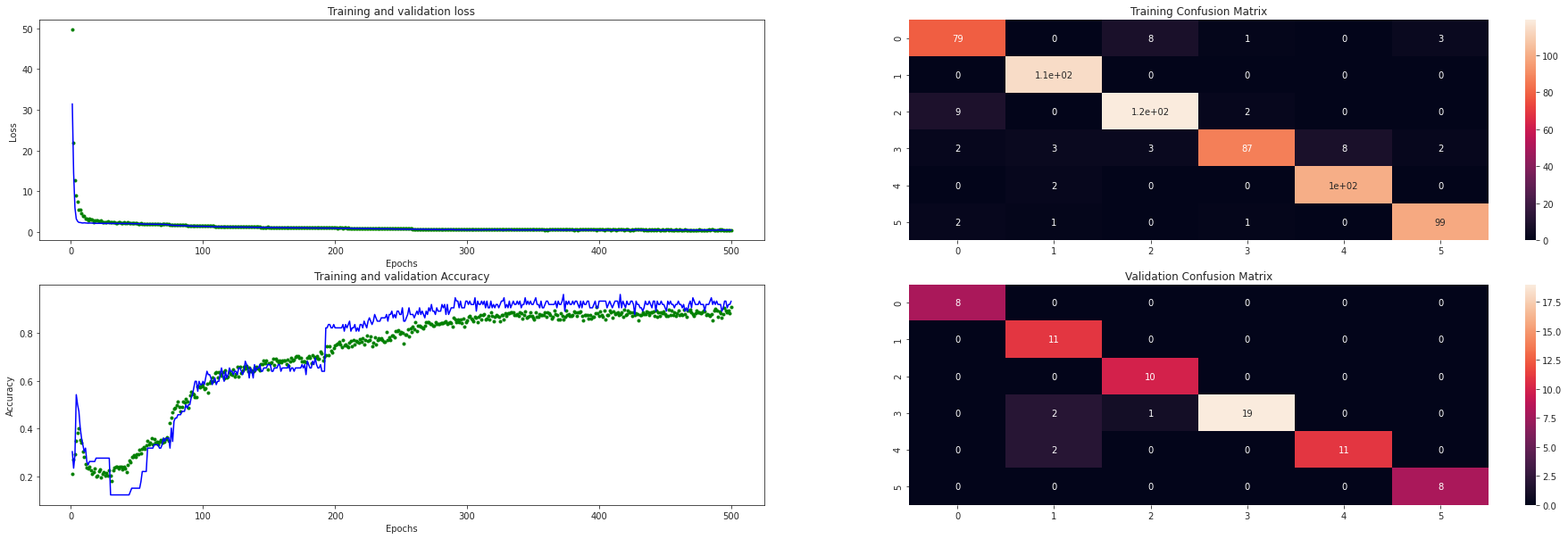
The following cell will loop through the training data num_iterations of times. Each time running a specific number of epochs. After each iteration, the visualizations for the loss, accuracy, and confusion matrix will be updated for both the validation and training data sets. You can use this to see how the model is progressing.
from IPython.display import clear_output
import sensiml.tensorflow.utils as sml_tf

num_iterations=1
epochs=100
batch_size=32


data  = tf.data.Dataset.from_tensor_slices((x_train, y_train))
shuffle_ds = data.shuffle(buffer_size=x_train.shape[0], reshuffle_each_iteration=True).batch(batch_size)

for i in range(num_iterations):
    history = tf_model.fit( shuffle_ds, epochs=epochs, batch_size=batch_size, validation_data=(x_validate, y_validate), verbose=0)

    for key in train_history:
        train_history[key].extend(history.history[key])

    clear_output()
    sml_tf.plot_training_results(tf_model, train_history, x_train, y_train, x_validate, y_validate)
Quantize the TensorFlow Model
Now that you have trained a neural network with TensorFlow, we are going to use the built-in tools to quantize it. Quantization of NN allows use to reduce the model size by up to 4x by converting the network weights from 4-byte floating-point values to 1-byte uint8. This can be done without sacrificing much in terms of accuracy. The best way to perform quantization is still an active area of research. For this tutorial, we will use the built-in methods that are provided as part of TensorFlow.
The
representative_dataset_generator()function is necessary to provide statistical information about your dataset in order to quantize the model weights appropriately.The TFLiteConverter is used to convert a TensorFlow model into a tensor flow lite model. The TensorFlow lite model is stored as a flatbuffer which allows us to easily store and access it on embedded systems.
import numpy as np
def representative_dataset_generator():
    for value in x_validate:
    # Each scalar value must be inside of a 2D array that is wrapped in a list
        yield [np.array(value, dtype=np.float32, ndmin=2)]
# Unquantized Model
converter = tf.lite.TFLiteConverter.from_keras_model(tf_model)
tflite_model_full = converter.convert()
print("Full Model Size", len(tflite_model_full))

# Quantized Model
converter = tf.lite.TFLiteConverter.from_keras_model(tf_model)
converter.optimizations = [tf.lite.Optimize.OPTIMIZE_FOR_SIZE]
converter.representative_dataset = representative_dataset_generator
tflite_model_quant = converter.convert()

print("Quantized Model Size", len(tflite_model_quant))
INFO:tensorflow:Assets written to: /tmp/tmplq8x91qn/assets
INFO:tensorflow:Assets written to: /tmp/tmplq8x91qn/assets
Full Model Size 3128
INFO:tensorflow:Assets written to: /tmp/tmpd_z6dko0/assets
INFO:tensorflow:Assets written to: /tmp/tmpd_z6dko0/assets
Quantized Model Size 3088
An additional benefit of quantizing the model is that TensorFlow Lite Micro is able to take advantage of specialized instructions on Cortex-M processors using the cmsis-nn DSP library which gives another huge boost in performance. For more information on TensorFlow lite for microcontrollers, you can check out the excellent tinyml book by Pete Warden.
Uploading the TensorFlow Lite model to SensiML Cloud
Now that you have trained your model, it’s time to upload it as the final step in your pipeline. From here you will be able to test the entire pipeline against test data as well as download the firmware which can be flashed to run locally on your embedded device. To do this we will use the Load Model TF Micro function. We will convert the tflite model and upload it to the SensiML Cloud server.
Note: An additional parameter that can be specified here is the threshold. We set it to .1 in these examples. Any classification with a value less than the threshold will be returned as theunknownclassification.
class_map_tmp = {k:v+1 for k,v in class_map.items()} #increment by 1 as 0 corresponds to unknown

client.pipeline.set_training_algorithm("Load Model TF Micro",
                                    params={"model_parameters": {
                                            'tflite': sml_tf.convert_tf_lite(tflite_model_quant)},
                                            "class_map": class_map_tmp,
                                            "estimator_type": "classification",
                                            "threshold": 0.0,
                                            "train_history":train_history,
                                            "model_json": tf_model.to_json()
                                            })

client.pipeline.set_validation_method("Recall", params={})

client.pipeline.set_classifier("TF Micro", params={})

client.pipeline.set_tvo()

results, stats = client.pipeline.execute()
Model Summary
After executing the pipeline, the cloud computes a model summary as well as a confusion matrix. The model summary gives a quick overview of the model performance so we can see what the accuracy of the quantized model was across our data set.
results.summarize()
TRAINING ALGORITHM: Load Model TF Micro
VALIDATION METHOD:  Recall
CLASSIFIER:         TF Micro

AVERAGE METRICS:
                 F1_SCORE:  92.6  std: 0.00
                PRECISION:  92.8  std: 0.00
              SENSITIVITY:  92.7  std: 0.00

--------------------------------------

RECALL MODEL RESULTS : SET VALIDATION

MODEL INDEX: Fold 0
                 F1_SCORE:    train: 92.64  validation: 92.64
              SENSITIVITY:    train: 92.71  validation: 92.71
Confusion Matrix
The confusion matrix provides information not only about the accuracy but also what sort of misclassifications occurred. The confusion matrix is often one of the best ways to understand how your model is performing, as you can see which classes are difficult to distinguish between.
The confusion matrix here also includes the Sensitivity and Positive Predictivity for each class along with the overall accuracy. If you raise the threshold value, you will notice that some of the classes start showing up as having UNK values. This corresponds to an unknown class and is useful for filtering out False Positives or detecting anomalous states.
model = results.configurations[0].models[0]
model.confusion_matrix_stats['validation']
CONFUSION MATRIX:
               Cross      Hook       Jab   Unknown  Uppercut  Overhand       UNK       UNC   Support   Sens(%)
     Cross      87.0       0.0      10.0       2.0       0.0       1.0       0.0       0.0     100.0      87.0
      Hook       0.0     125.0       0.0       6.0       3.0       1.0       0.0       0.0     135.0      92.6
       Jab       8.0       0.0     129.0       4.0       0.0       0.0       0.0       0.0     141.0      91.5
   Unknown       1.0       0.0       2.0     106.0       0.0       1.0       0.0       0.0     110.0      96.4
  Uppercut       0.0       0.0       0.0       8.0     111.0       0.0       0.0       0.0     119.0      93.3
  Overhand       3.0       0.0       0.0       2.0       0.0     107.0       0.0       0.0     112.0      95.5

     Total        99       125       141       128       114       110         0         0       717

PosPred(%)      87.9     100.0      91.5      82.8      97.4      97.3                        Acc(%)      92.7
Finally, we save the model knowledge pack with a name. This tells the server to persist the model. Models that you persist can be retrieved and viewed in the Analytics Studio in the future. Models that are not saved will be deleted when the pipeline is rerun.
model.knowledgepack.save("TFu_With_SensiML_Features")
Knowledgepack 'TFu_With_SensiML_Features' updated.
Testing a Model in the Analytics Studio
After saving your model, you can return back to the Analytics Studio to continue validating and generating your firmware. To test your model against any of the captured data files, select the pipeline and
Go to the Explore Model tab of the Analytics Studio.
Select the pipeline you built the model with.
Select the model you want to test.
Select any of the capture files in the Project.
Click RUN to classify that capture using the selected model.
The model will be compiled in the SensiML Cloud and the output of the classification will be returned. The graph shows the segment start and segment classified for all of the detected events.
Running a Model On Your Device
Downloading the Knowledge Pack
Now that we have validated our model it’s time for a live test. To build the firmware for your specific device go to the Download Model tab of the Analytics Studio. We support compiled binaries for our target platforms which include fully configured sensors and classification reporting over BLE. We also provide compiled libraries that can be integrated into your application. For enterprise customers, you will have full access to the SDK and can take the compiled models and modify or optimize them for your target devices.
If you are using Community Edition you can download the firmware binary for your device. SensiML customers are able to download library and source code as well. Head over to the Analytics Studio to download your model and flash it to the device. To download the firmware for this tutorial
Go to the Download Model tab of the Analytics Studio
Select the pipeline and model you want to download
Select the HW platform Quicklogic S3AI Chilkat 1.3
Select Format Library
To turn on debug output check Advanced Settings and set Debug to True
Click on Output and add Serial as an option as well which enables uart output over serial
Click Download and the model will be compiled and downloaded to your computer ready to flash.
After downloading the Knowledge Pack, follow the instructions associated with your firmware for flashing it. We have flashing instructions for our supported boards here.
Live Test Using SensiML TestApp
Being able to rapidly iterate on your model is critical when developing an application that uses machine learning. In order to facilitate validating in the field, we provide the SensiML TestApp. The TestApp allows you to connect to your microcontroller over Bluetooth and see the classification results live as they are generated by the microcontroller.
The TestApp also has some nice features, such as the ability to load the class-map, associate images with results, see the history, and apply a majority voting post-processing filter. Documentation on how to use the TestApp can be found here. In this example, we have loaded the TestApp with images of the different punches our glove performs, as we perform the punch, the results will be displayed in the TestApp along with the picture and class name.
Summary
We hope you enjoyed this tutorial using TensorFlow along with SensiML Analytics Toolkit. In this tutorial we have covered how to:
Collect and annotate a high-quality data set
Build a feature extraction pipeline using SensiML
Use TensorFlow to train a NN to recognize different punch motions
Upload the TensorFlow Lite model to SensiML Cloud and download the Knowledge Pack firmware.
Use the SensiML TestApp to perform live validation of the model running on the device.
For more information about SensiML visit our website. To work with us to enable you to build your application get in touch with us or send an email to info@sensiml.com.
SensiML
SensiML enables developers to quickly and easily create machine learning models that run locally on resource-constrained edge devices. SensiML SaaS provides an end to end solution from collecting and annotating a high-quality sensor time-series data set, to analyzing and building data models using AutoML, and finally generating firmware that will run on your target device.
TensorFlow Lite for Microcontrollers
TensorFlow Lite for Microcontrollers is a port of TensorFlow Lite designed to run machine learning models on microcontrollers and other devices with only kilobytes of memory. It implements a limited subset of TensorFlow operations but is more than enough to build high accuracy models for running efficient inference on resource-constrained devices.