Robot Arm Motion Recognition and Anomaly Detection
Overview
Robotic applications are typically programmed with proprietary software specific to the given system, often using what is known as a teach pendant to define motion paths, end-of-arm tooling commands, and other key events. When all goes well, the robotic arm performs tasks as planned per the recipe programmed. But what about when unexpected external events occur? The repercussions of an accidental robotic collision with nearby workers, unexpected machine conditions, and environmental anomalies can have serious productivity, quality, and worker safety consequences. This application showcases an ML-trained, motion analysis device that can operate independent of the monitored robotic system to alert in real-time to anomalies such as:
Unprogrammed movements
Mechanical faults
Unexcepted collisions
Human interference or obstruction
Environmental changes
Robot Preparation
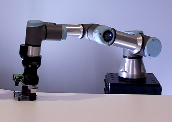
Assemble the robot and load the desired program. For this document, we use a Universal Robot Arm provided by onsemi. However, the following instructions can be used to build motion path recognition models for other type of robot arms.
Load the robot program, i.e., sensors_converge_2.urp. In this program, robot starts from a standing position and reaches to its base to pick a cube. Then it moves back to a partially standing position and rolls back and forth before it reaches to the same location and put the cube on the same spot and goes back to its original standing position.
Flash the SensiML data capture firmware on the onsemi RSL10 Sense device mounted on top of the robot head. For additional information on how to properly communicate with the onsemi RSL10, please refer to the SensiML Documentation.
Data Collection
You need to have the SensiML Data Studio in order to record data
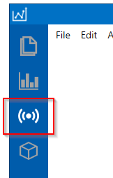
Create a new project and click the Live Capture button in the left navigation bar
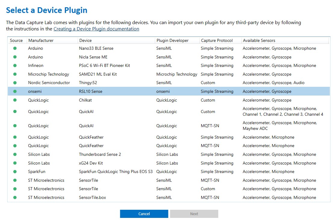
Select the onsemi RSL10 Sense configuration from the device menu
In this tutorial, we use the sampling rate of 100/seconds.
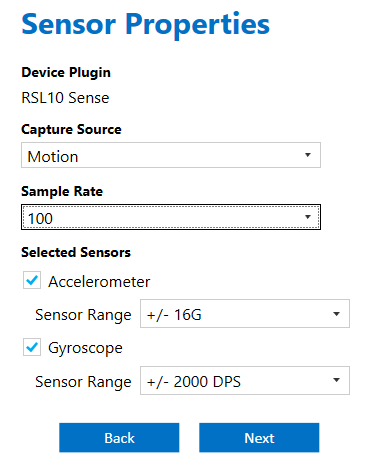
Connect to the onsemi RSL10 Sensor. If successful, six motion signals (3 accelerometers and 3 gyroscopes) will begin streaming to the Data Studio.
Move the robot arm to its beginning position, but do NOT play the program yet.
In the Data Studio, set your desired file name properties and press the “Start Recording” button to start recording the signal.
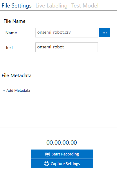
Wait for the robot to complete a few full cycles. After the cycles are complete, wait for the robot to reach its standing position and then stop recording the signal.
Optional: You can connect to a camera in the Data Studio and record video of the robot with the signal. Later this may help you annotate the signal.
Note: Repeat this process for 4-5 files.
Data Annotation
Labels
There are 6 different labels in the sensors_converge_2.urp program
In the Data Studio main menu, open Edit > Project Properties > Segment Labels and define the proper labels for these motions
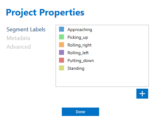
For this program, we end up with six labels
Approaching: Robot moves from its standing position towards the cube
Picking_up: Robot picks up the cube and moves back to a standing position
Rolling_right: While holding the cube, the robot head rolls to its right side
Rolling_left: While holding the cube, the robot rolls back to its left side
Putting_down: The robot goes back to the original location of the cube and puts it back on the same spot
Standing: After putting down the cube, the robot goes back to its original standing position
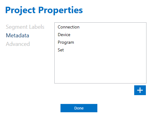
Metadata
In the Project Properties, you can also define custom metadata to describe your files. You may want to keep track of the name of the robot program, the purpose of the data set (for example if used for training or testing), the sensor device, etc.
Annotation Session
The Data Studio uses labeling “Sessions” to have a way of version controlling and organizing the project. Users will add “Segments” which are the labeled events in a file to a “Session”.
“Sessions” can be either “manual” or “automatic”. In “manual” sessions, users are able to add segments manually by clicking on different regions of the signal. In “automatic” sessions, users are able to use a segmenter algorithm to automatically label the regions of the signal.
For this tutorial, we will use an automatic session.
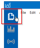
Open the Project Explorer in the left navigation bar to view the files in your project.
Open a file by double-clicking on the file in the list.
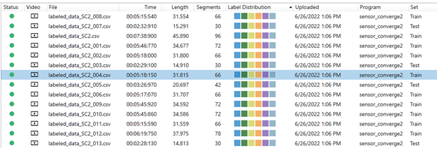
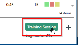
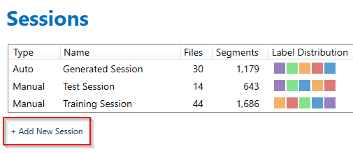
View the sessions in your project by clicking on the session name in the bottom right corner of the Project Explorer.
Click Add New Session to create a new labeling session
Enter a name for your session and select “Auto”.
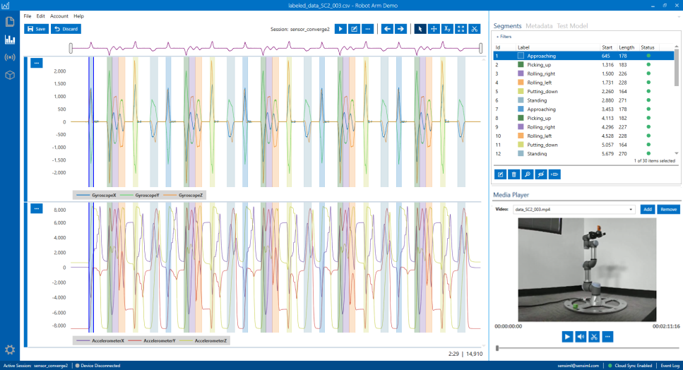
Select “General Threshold Segmentation” as the segmenter algorithm and set other parameters according to the following screenshot.
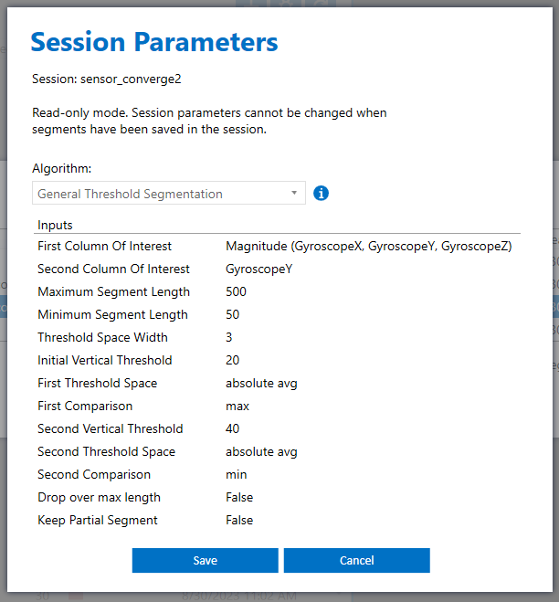
The beginning of the segment will be determined based on the “First Column of Interest” property, which is the Gyroscope magnitude calculated from its cardinal components. In our example, the absolute average of the Gyroscope magnitude must be greater than the Initial Vertical Threshold size of 20 within the Threshold Space Width (sliding window) size 3 samples.
In this project, we determine the ending of a segment based on where the absolute average of GyroscopeY signals drops below a threshold value 40 within the Threshold Space Width (sliding window) size 3 samples.
Note
Finding the best parameters to use in your segmenter algorithm requires some experimentation. You can use the “detect segments” button to try out the segmenter algorithm and make proper adjustments to detect all segments. The rule of thumb for robot movements is to confine segments based on combinations of Gyroscope signals. The associated accelerometer data can be later picked by the ML model for recognition purposes.
Once all your desired segments are recognized, you can set their labels accordingly.
Adding segments to files can also be accelerated by using your own tools for labeling outside of the Data Studio (for example using a Python script to label a file). You can import/export labels through an open format we call the DAI format. You can export segments to the DAI format by selecting a list of files in the “Project Explorer” -> Right + Click -> Export. The DAI file can be updated with the appropriate labels that are ordered periodically mimicking the robot cycles. The updated DAI file could be imported back to the Data Studio project to update the labels of the capture files. To update the DAI file, you can use any programming language of your choice.
Building the Motion Recognition Model
The motion recognition model can be generated in the SensiML Analytics Studio. Login to your account and open the project.
The steps are as follows
Adding a query
Creating a model pipeline for the AutoML engine
Optimizing the model
Testing the model
Adding a Query
The first step in generating a model is to extract the right segmented data with the appropriate annotations. You can use a combination of data columns, metadata, sensor sources, and label groups to filter out the data you need for your model. Here, we assume the underlying collected data for the robot program “sensors_converge_2.urp” have been annotated in the Data Studio in the session “sensor_converge2”.
Click on the “Prepare Data” menu item on the left side of the Analytics Studio.
To create a new query
Click on the “Add New Query”
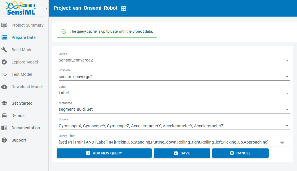
Fill in the query form to extract your desired data
Query: Choose a name for your query
Session: Select the session you used in the Data Studio to segment and annotate your data
Label: Select the label group
Metadata: Choose all the metadata items you want to use to filter the data for your model. For example, if you are tracking the Training and Testing datasets in the “Set” column, you choose the column “Set” along with other metadata columns that you need
Source: Select all sensors that you want to build your model based upon
Query Filter: Click on edit triangle-shape icon on the right and put your desired fields and criteria to filter out the data. For instance, we use the “Set” metadata column to extract the “Training” data to build our model
Save the query
Building a Pipeline
To build a model, first you need to generate a pipeline that extracts the desired data segments by running the corresponding query. Each pipeline also contains a set of instructions to convert each segment to a set of features that are used in multiple machine learning algorithms.
The SensiML AutoML engine explores multiple combinations of ML algorithms with different features. The 5 best models are then returned based on the adopted evaluation metrics.
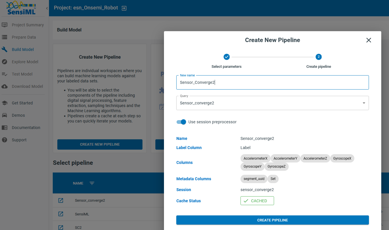
To begin building a pipeline, go to the “Build Model” from the left menu. Name your pipeline and choose the query you have prepared previously from the drop-down menu. Activate “Use session preprocessor” to ensure that the segmenter algorithm is invoked to automatically parse the signal prior to the recognition model. This segmenter algorithm is the one you used for generating segments and annotation them in the Data Studio (see here). Therefore, it is vital that the parameters of an automatic segments are accurately adjusted to be only sensitive to the motion profiles of interest.
Click on the “Create Pipeline” button to start shaping your pipeline.
Pipeline Steps
A pipeline consists of a series of steps that act as the instructions for building a model.
A brief description of each of the steps in a pipeline can be found below:
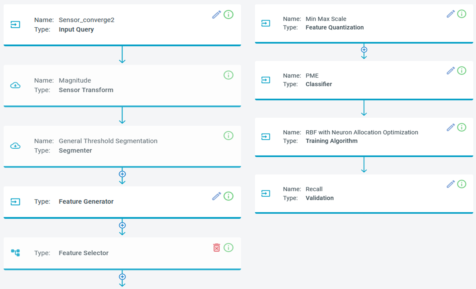
Input Query: a set of criteria to prepare the desired captured data for the pipeline. Use the query you created earlier.
Sensor Transformation: preprocessing the data segments, such as calculating the magnitude of the acceleration vector from its three components. Activating the “use of session preprocessor” invokes the corresponding transformations associated to the session
Segmenter Algorithm: the procedure to extract segments of data. This can be the same as the segmenter used in an automatic session in the Data Studio, or a different algorithm such as “windowing” that generates segments of the specified window size. Switching to the “use of session preprocessor”, the same algorithm is used to generate data segments for the pipeline. The same algorithm is used when running the final model on an embedded device in live mode
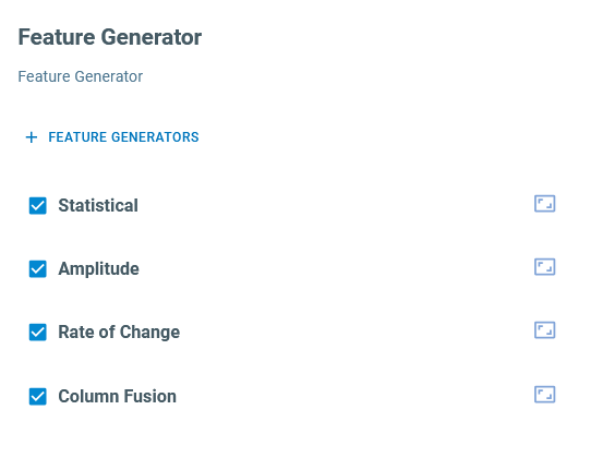
Feature Generator: uses different methodologies to extract various features from the data segments. Users might specify a set of feature generators that significantly describe the data behavior or the AutoML algorithm to find the best combination.
Click on the “edit” button on the top right side of this block to add or remove features. For this application, we use four family of generators and let the AutoML engine find the most relevant combination
Statistical Features: to extract statistical information about the signal such as mean, median, skewness, kurtosis, percentiles etc.
Amplitude: to compute features from the amplitudes of signals, such as global min/max sum, global peak-to-peak
Rate of Change: to monitor how signals change with time
Column Fusion: to combine the information of different sensors
Feature Selector: a set of methods to select the most relevant features
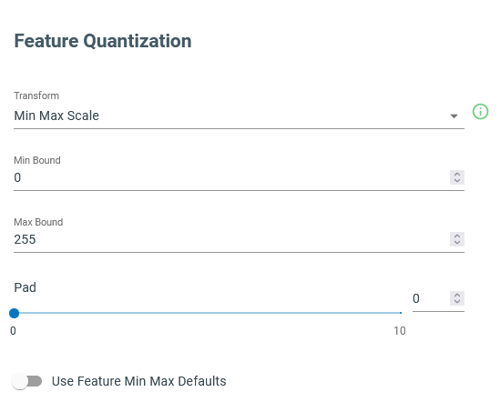
Min/Max Scaling: scaling the chosen features to make them compatible with the memory criteria of the embedded devices. For instance, for 8-bit devices, all features are mapped into the 0-255 range.
Classifier: the machine learning algorithm that takes the scaled features and generates classifications. Click on the edit button of the panel to modify the underlying parameters.
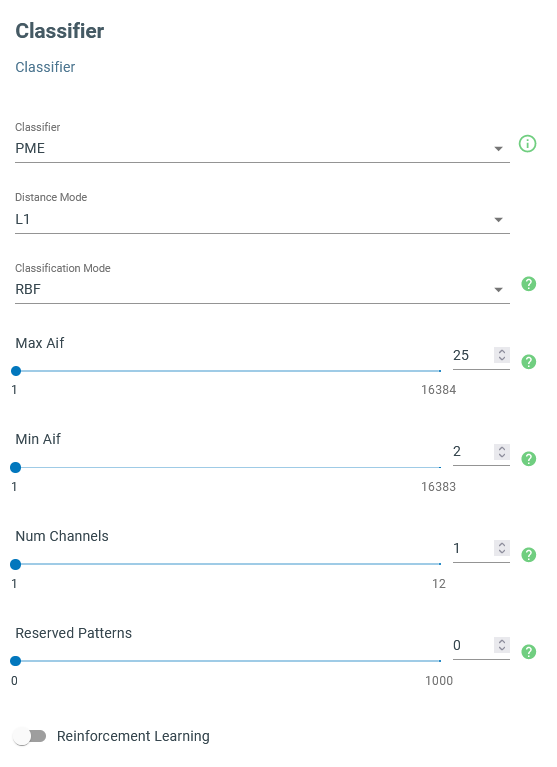
For this application, we use “Pattern Matching Engine” (PME) to generate classifications. In this scenario, the distances between the feature vector and a set of predetermined patterns in the feature space are calculated and used for classification. We use the “L1” metric to calculate distances and the “RBF” algorithm to generate classifications.
“RBF” takes advantage of a set of patterns whose sizes are constrained by Max/Min AIF (the size of influence fields). If an input feature vector falls outside all influence fields, the signal is classified as anomalous and “unknown” is returned as the output class. One must change the minimum and maximum sizes of influence fields to make sure all known signals are classified correctly while erroneous signals are not misclassified. It is suggested to set the Max Aif to very large values to get reasonable results and then gradually reduce that value to increase the sensitivity to the unusual signals.
In the case of the robot arm movements, the abnormal signals might be generated when the robot collides with an obstacle or some of its motors are no longer moving as expected, that make this algorithm useful for both collision detection and predictive maintenance applications.
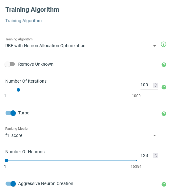
Training Algorithm: the method to train the machine learning algorithm.
Use “Neuron Allocation Optimization” to train the PME-RBF algorithm. You may leave the other parameters unchanged and evaluate the final resulting models. Changing the number of neurons affects the final performance of the model. More neurons create more complex models that are prone to overfitting, although, at the same time it allows us to more efficiently investigate higher dimensional feature spaces which might imply increasing the sensitivity to the anomalous signals.
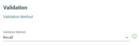
Validation Strategy: the instruction of how to split data into training and validation sets.
Here, we use “Recall” for the validation method meaning that the entire training set is taken for the model evaluation process and construction of the confusion matrices.
Pipeline Settings: a set of parameters to control the AutoML workflow, such as the number of iterations, the performance metric(s), the ML models to be explored, etc.
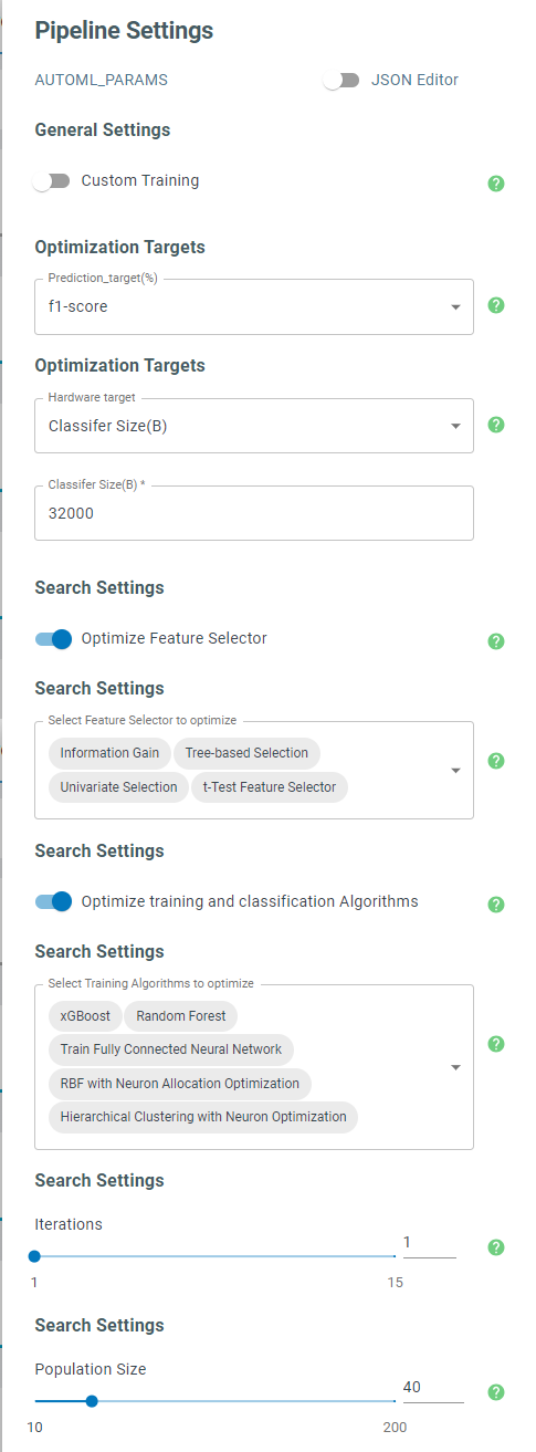
The AutoML engine explores candidate features and ML algorithms to find the best combination that optimizes the objective metric. For this application however, we have already set the classifier and training algorithms. Therefore, we deactivate the optimization of the training and classification algorithms and only let AutoML optimize the feature selector.
The optimization algorithm generates ensembles of models generated randomly and evolves them by eliminating the lowest relevant features and removing models that exhibit weak performances. This evolutionary algorithm cycles through several iterations to replace low performance models with more promising models by mutating their characteristics. In the end, the top five best candidates are returned. “Population Size” specifies the extent of the original pool of models. An accepted model needs to go through the specified number of “Iterations” to make it to the final list. The larger population and cycling through more iterations usually help with finding better results owing to spanning larger regions in the feature space.
Note
To better detect the abnormal robot movements, it is suggested to tweak the pipeline parameters to end up with models that use relatively more features yet display acceptable performances. Lower the maximum area of the influence field of the PME classifier to a point that does not cause the models to downgrade.
Testing and Deploying
The AutoML algorithm offers 5 of the best models that pass all your criteria. If you run the algorithm several times, you may end up with slightly different models, because each time the initial model pool is constructed randomly.
Click on the “Explore Model” in the left menu and choose one of the models with highest accuracy and larger number of features.
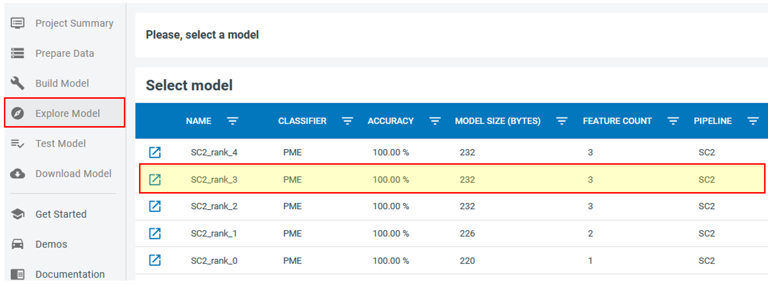
Click on  to expand the model and explore its properties, such as the confusion matrix and the selected features. Note that for the robot arm demo, although the automatic segmenter has been fully constructed based on the gyroscope signals we still want to end up with classification models that take advantage of the accelerometer signals as well.
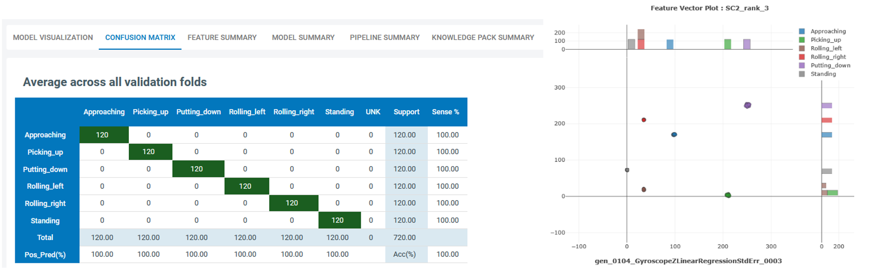
The following diagram shows the confusion matrix for the highlighted model in the top figure (left) and the 2-dimentaional visualization of two of its features (right). As seen, adopting only two features this model can achieve the accuracy of 100%, however, adding extra redundancy helps with the model robustness and more confidently singling out the anomalous behaviors.
Running a Model on Files in the Data Studio
The Data Studio can run models on any CSV or WAV file that you have saved to your project in the Project Explorer.
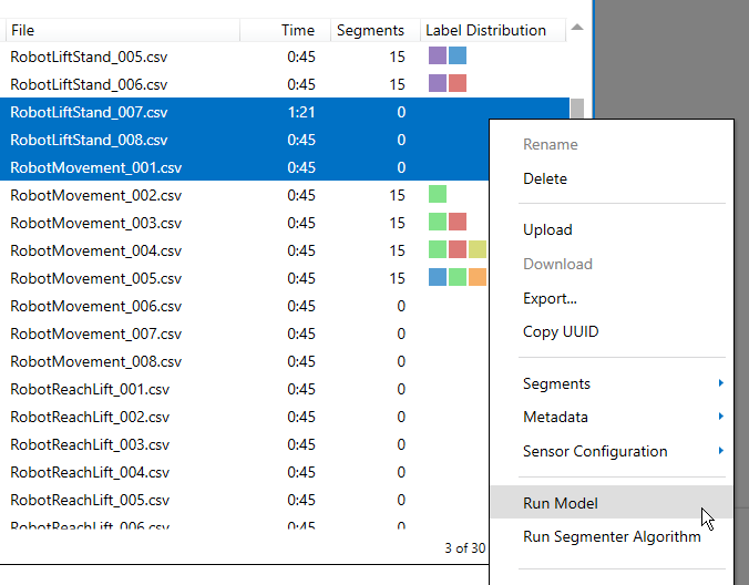
Open the Project Explorer in the left navigation bar.
Select the files you have reserved for the testing purpose and Right + Click > Run Model.
You can then compare your model results with your training data. This is a good way to evaluate the power of the model to associate the relevant segments with the right labels.
Running a Model in Real-Time in the Data Studio
The Data Studio can graph model results in real-time with your data collection firmware.
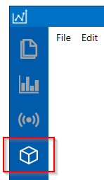
Click on the Test Model button in the left navigation bar.
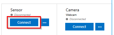
Connect to your onsemi RSL10 Sense device that is mounted on the robot to stream the data.
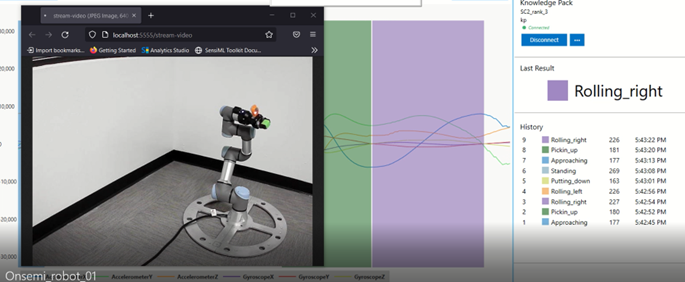
Select a Knowledge Pack to start recognizing the signal as the robot moves.
You can observe the movements of the robot arm and evaluate the performance of the model as it classifies each move. You can introduce some anomalies by disturbing the robot motion or running a different program. A good model must capture most of the abnormal activities.
Running a Model in Real-Time on a Device
You can download the compiled version of the Knowledge Pack from the Analytics Studio and flash it to your device firmware.
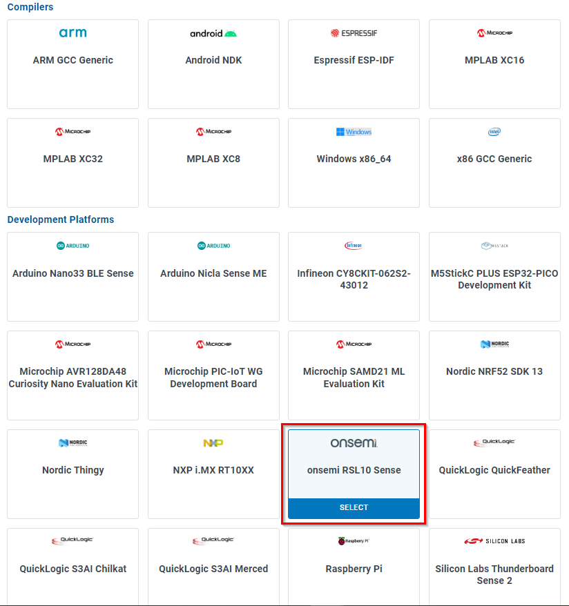
Open the Download Model page.
Select your platform. For this guide we are using the onsemi RSL10 Sense. Instructions for flashing the onsemi RSL10 Sense can be found in the onsemi RSL10 Sense Firmware Documentation
Instructions on flashing other supported platforms can be found in the Flashing a Knowledge Pack to an Embedded Device Documentation
Instructions on integrating Knowledge Pack APIs into your firmware code can be found in the Building a Knowledge Pack Library Documentation
To see classification results, use a terminal emulator such as Tera Term or the SensiML Open Gateway.