
Opportunities to improve manufacturing processes by adding machine learning sensors at the IoT edge are rapidly emerging. Thanks to a combination of
- Powerful microcontrollers and multi-core SoCs like the EOS S3 on QuickLogic’s QuickAI HDK
- High-resolution, low-cost MEMS sensors and microphones
- Powerful AutoML-based AI tools like SensiML Analytics Toolkit
it is possible to bring sophisticated machine learning analysis to industry-specific processes and even accommodate machine-to-machine level ML model tuning.
Typically, Industrial IoT (IIoT) and smart connected factory projects focus on macro-level process insights using centralized cloud or edge server analysis combined with a scalable network of hundreds to thousands of basic sensors like limit switches, temperature alarms, speed sensors, and other simple inputs. More complex sensors tend to overtax centralized analytics to the breaking point with an avalanche of raw data that is expensive to transport and process.
But adding local IoT endpoint ML analytics to these more complex sensors changes the game by transforming high sample rate physical sensors to application-specific basic sensors tailored to a specific set of metrics of interest for a given process. Imagine the possibilities for improved visibility and control with the addition of machine-specific pattern recognition for audio, vision, vibration, pressure, force, strain, current, voltage, and motion sensing using local AI processing. Such powerful real-time insight has only recently become practical.
Along these lines, SensiML is supporting researchers at Taiwan’s National Kaohsiung University of Science and Technology (NKUST) with software for building practical applications of IoT smart sensing for real-world industrial processes. The case study that follows highlights one such application of smart sensing NKUST undertook for monitoring the mold status of injection molding processes.
In the diagram below, we can see a variety of components that make up the injection molding process, each of which can benefit from the insights of smart IoT edge sensing.

Let’s break these down into specific insights of interest:
- Drive Motor: Is the motor behaving properly? Vibration sensing can detect bearing degradation, current/voltage/shaft encoder can reveal anomalous operating profiles, power degradation, and mechanical faults.
- Injection Cylinder: Is the injection charge flowing as expected? Pressure versus cylinder dispalcement profiles can reveal jammed extruder screws, improper heating, viscosity issues, and mold flow problems
- Mold Cavity: Are the parts forming well and ejecting correctly? Acoustic and vibration monitoring of the mold itself can provide insights on proper mold closure/seal, injection fill, short shots, excess flashing, and proper part ejection
What follows is an article, originally published by MakerPro, that has been adapted and translated here to describe the first in a series of models NKUST is creating to showcase the potential for smart IoT sensing in the field of injection molding.
AI at the IoT Edge Realization on the Production Line – An Injection Molding Machine Example
Author: Kang Zhiwei,
Chief Editor: Xie Hanru
Further adaptation and editing for SensiML.com by Chris Rogers
Original article: https://makerpro.cc/2021/07/mcu-based-machine-learning-case-study/
In recent years, advancing needs and technological progress have brought many advances to manufacturing. The recent major transformation of the industry occurred in the Industry 4.0 project initiated by the German government in 2011, with the purpose of Advance the overall industrial production pattern from the original automation to the intelligence. The core technologies related to Industry 4.0 are developing rapidly, such as the Internet of Things (IoT), Cloud (Cloud), Big Data, Artificial Intelligence (AI), and robotics.
Among them, the development and application of artificial intelligence in recent years has created many new training methods and algorithms in response to the different needs of the field. The most frequently discussed in the field of artificial intelligence are machine learning and deep learning.
Machine learning can be roughly divided into three aspects:
- Supervised Learning
- Unsupervised Learning
- Reinforcement Learning
The principle of supervised learning is used in this article and relies on the annotation of data features and corresponding data training methods to build classification models. This article focuses on the application of annotated supervised ML data to processes used in the mold industry, specifically with injection molding machines and the use of acoustic sensors to collect the audio samples of the machine during production use for real-time analysis using supervised ML methods. We will focus on the mold itself and seek to predict events for mold closure, the injection process, and mold ejection using acoustic signatures.

The ML method involves labeling and training various machine states to produce a predictive AI model that can automatically identify the production status of the machine. This prediction result is then received in real-time through a computer or a smart handheld terminal device so that a complete Internet of Things system is formed between the production machine, the sensor, the smart handheld terminal device, and the computer. What follows is a detailed explanation of the overall experimental process and hardware and software configuration to accomplish this goal.
The Hardware Setup
The sensor used in this article is QuickLogic’s Merced HDK (Hardware Development Kit). This development version is very suitable for the next generation of low-power machine learning IoT devices. At the same time, the Merced HDK is equipped with a 16KHz ODR digital microphone, electronic compass, and six-axis inertial measurement unit (three-axis gyroscope and three-axis accelerometer).
The digital microphone used in this article is SPH0641LM4H manufactured by Knowles, which has the characteristics of miniature, high performance, and low power consumption. The SNR of this component is 64.3 dB, the sound pressure level is 94 dB, and the sensitivity is -26 dB. The communication cable required to flash the model is Sabrent’s Type-A to Micro USB-B transmission cable. The smart handheld terminal device uses the ASUS ZenFone 5 with Android OS to support SensiML’s TestApp, a real-time model testing tool showing the inference output and other model details.
The Software Setup
Speaking of the SensiML tools, this article uses three applications that comprise the SensiML Analytics Toolkit suite to carry out the overall experiment. The first is the Data Capture Lab which is responsible for the collection, importing, raw data processing, and annotating of data features. The software can also import CSV and WAV format files for data processing and upload all the data to the cloud in real-time. From there, SensiML Analytics Studio uses a variety of algorithms and custom parameters to perform high-efficiency model generation (using what is known as AutoML – or machine learning to create machine learning models) based on the labeled data. Analytics Studio quickly produces high-performance edge computing models known as Knowledge Packs. Finally, these Knowledge Packs – once flashed to the hardware – can be monitored using SensiML’s debug/test tool known as TestApp. TestApp runs on the handheld device to verify and identify the production status of the machine through the connection with the sensor in real-time.
The Experiment
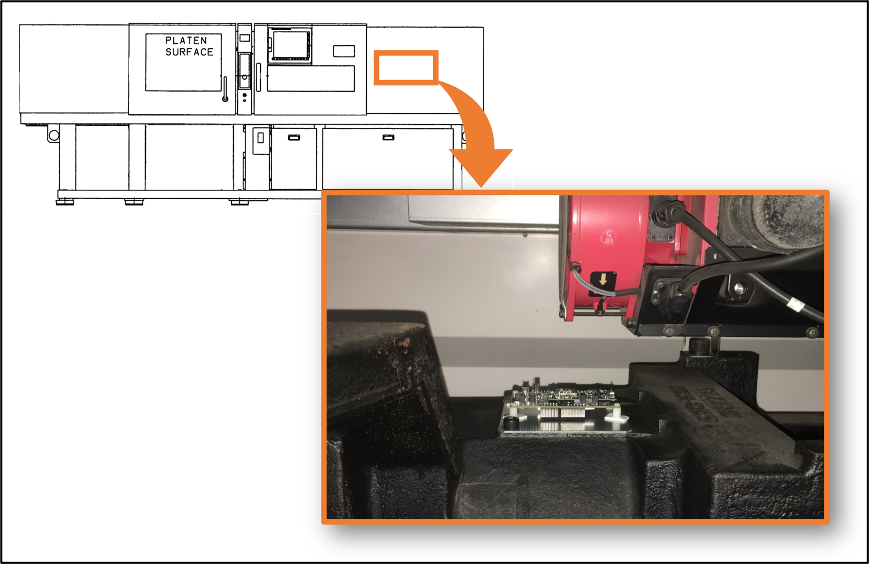
Step 1: Sensor Installation
After preparing the relevant hardware equipment and installing the required software/driver, you can start the experiment. First of all, we must install the sensor in a suitable location. Here we need to consider whether the ambient temperature of the installation location exceeds the operating temperature of the sensor and whether it hinders the production of machinery. This article finally chooses to install it on the shooter, as shown in Figure 3.
Step 2: Initial State Setting of the Sensor
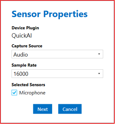
We open the Data Capture Lab application and create a project, then switch to Capture mode to add the initial sensor configuration, click the plus sign of Sensor Configuration to configure the device to the QuickLogic Merced HDK (QuickAI), use digital microphone components, and a sampling rate of 16 kHz as shown in Figure 4.
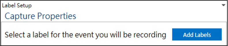
After successfully connecting with the sensor, we set the label we want to train, and click Add Labels to add a status label, as shown in Figure 5. For this application, we will establish labels for identifying the mold closing, injection, and ejection in the basic operation of the injection molding machine. There are three actions, so set Labels with the names of these three actions.
After setting up the Labels, you can start recording acoustic sensor data from the machine and select the appropriate label for the state being captured before recording, and then start recording (pictured left). Click Begin Recording to start recording (pictured); after recording, you can go to the Project Explorer to view the recording. The file (pictured right), will be named according to the label selected at the time of recording.

Step 3: Production Cycle Audio Recording
You can start recording audio after setting the required three labels of mold-off, injection, and ejection in the above steps. This article collects multiple complete production cycle audio samples, and the .qlsm/.wav file will be generated during the recording process. After importing into Data Capture Lab, it will be presented as an audio waveform, as shown in Figure 7. In addition, it can be converted to MFCC for comparison through commands.
Note: Mel-Frequency Cepstral Coefficients (MFCC)
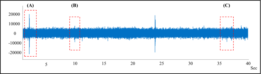
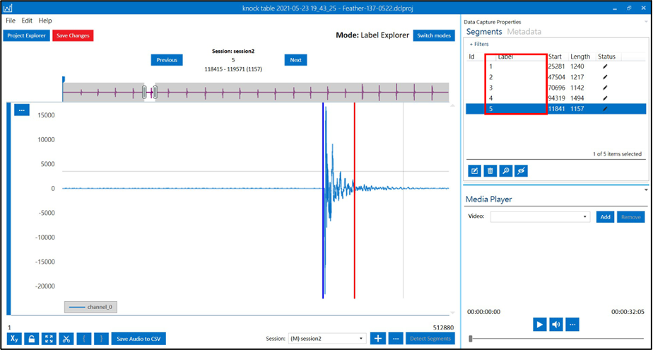
We can know from the cross-comparison between the audio and the actual video: (A) the mold is closed/sealed; (B) material is being injected; (C) completed mold part is being ejected, and the difference between the three can be clearly distinguished by zooming in on the waveform as shown in Figure 8.

Step 4: Annotate the Full Dataset
Then we can label all the previously recorded production audios, label the fragments we want to capture in Label Explorer mode, right-click to mark the segments of the spectral features to be recognized, and set the red box on the right to represent the feature. The label and annotation interface is shown in Figure 9.
Step 5: Model Training
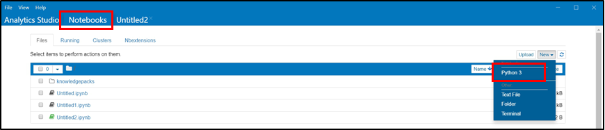
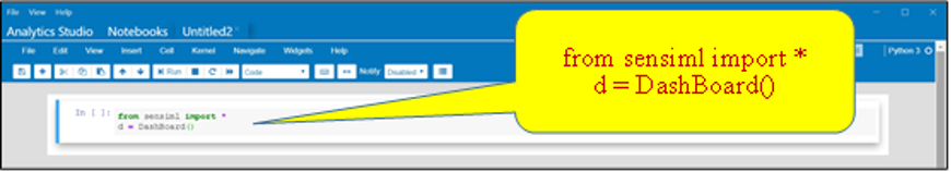
After marking the data segments of interest, we need to store and upload the dataset to the cloud and then train the model using Analytics Studio. First, we add a Python 3 project in the Notebook, as shown in Figure 10, and enter the code to run the training UI, as shown in Figure 11.
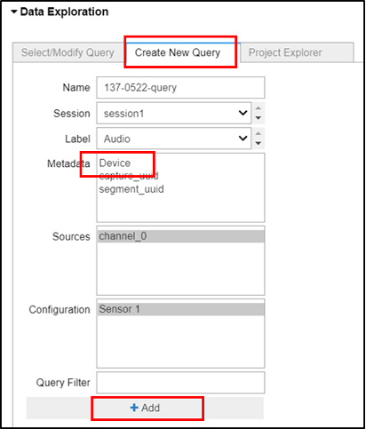
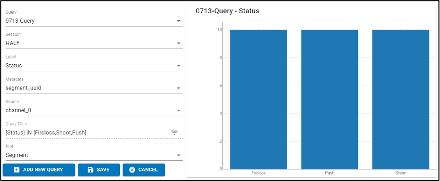
Then we select the project previously created in Data Capture Lab in Project, add a Pipeline name, and click Add, as shown in Figure 12. Then enter the name in Create New Query in Data Exploration and select Device and click Add, as shown in Figure 13.

At this stage, we have prepared all the data required for model training. After confirming that the label name on the right and the number of data items are correct, click Save to prepare and update the model training for the next step, as shown in Figure 14.
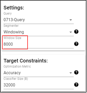
Model Building can be executed after the update. However, you need to pay special attention to the setting of the Window Size parameter, as shown in the red box in Figure 15, which can be understood as the size of the signal cutting interval. The value of this parameter needs to be appropriate to video and audio characteristics. Depending on discrete events or continuous events, this parameter will directly affect the accuracy of the overall model. After repeated experiments in this article, the best accuracy of 97% (96.88%) is obtained with 8000 units (representing a 500 msec window), as shown in Figure 16. From here, the power of the software is leveraged to perform AutoML model training which searches across many built-in algorithms to produce five candidate models at once, so we can select the most suitable model according to different needs.
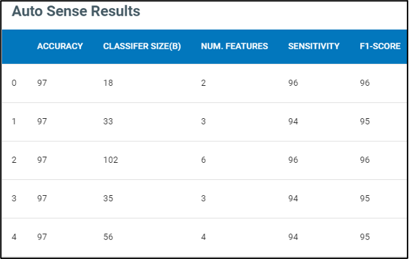
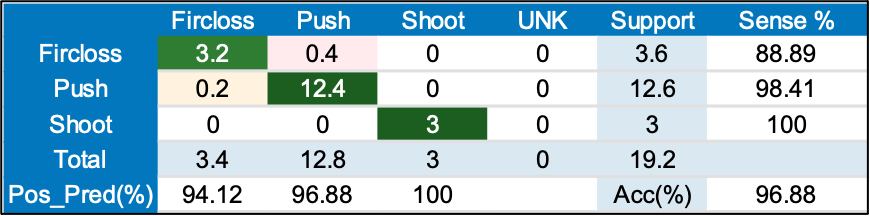
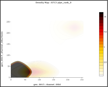
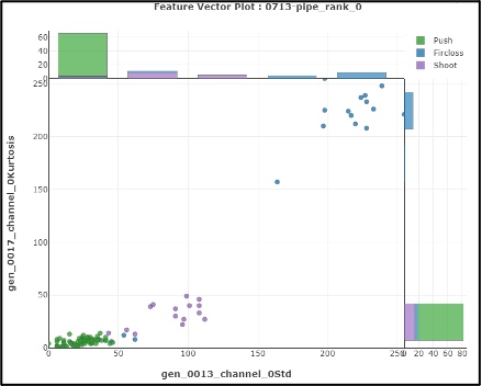
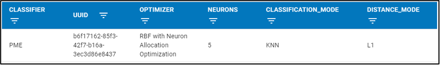
Once the model has been built, we can explore each of the candidate models in turn, reviewing indicators of the model in detail as in the confusion matrix shown in Figure 17. This article uses the classifier size, recall rate, and F1-Score evaluation indicators as references, and the number 0 model is selected as the optimal model. At the same time, we can further analyze the performance of the model through the vector graph or density map of the model, as shown in Figure 18 and Figure 19. This model uses K-NN for classification, as shown in Figure 20.
Step 6: Model Output and Flashing
After selecting the most suitable AI model, in order to apply it to the sensor, we must package and download the Knowledge Pack of the model, as shown in Figure 21.

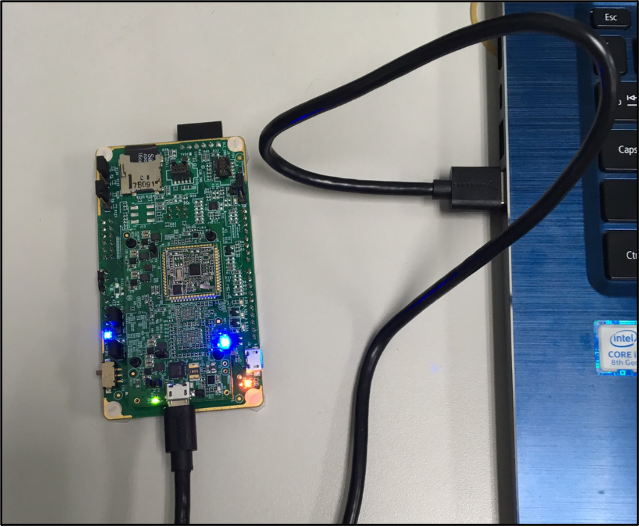
Then connect the sensor to the computer through the USB cable, and flash the .bin file of the above knowledge pack into the S3 AI chip. The connection and flashing configuration are shown in Figure 22 and Figure 23.
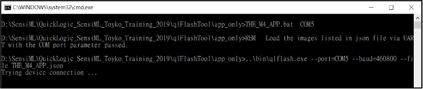
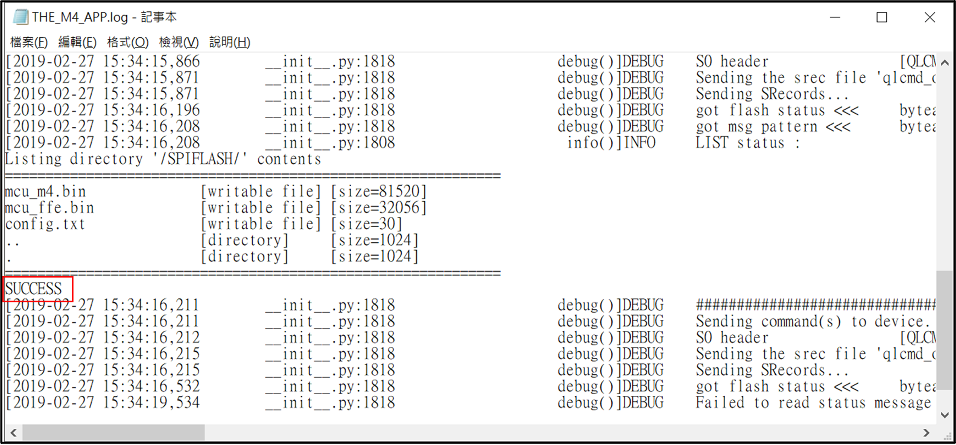
After the flashing is completed, you can enter the logs folder to watch the record. If Success appears, it means the flashing has been successful. The content of the Log is shown in Figure 24.
Step 7. Model verification
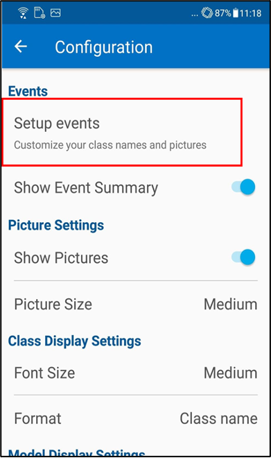
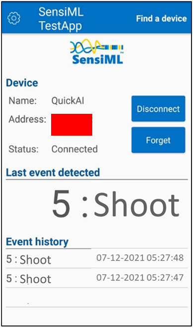
After successfully flashing the model into the sensor, we can then use the smartphone to verify whether the model is operating normally and receives the most real-time production status information. First, open SensiML TestApp and connect to the target sensor through Bluetooth, then enter Setup events and enter the label information of model.json in the previous Knowledge Pack into the fields, as shown in Figure 25. After the tag status setting is completed, if the sensor is operating normally and successfully recognizes the production status of the machine, the status will be updated immediately in the last event detected, as shown in Figure 26.
Summary
Since the development of artificial intelligence, there have been many software and hardware operations that become accessible to those without AI expertise and achievable on hardware at the smallest scale. This has the advantage of allowing users to focus more on the application of machine learning and not get mired in the details of the algorithms themselves. This article only uses the digital microphone unit on the QuickLogic Merced HDK. Many additional sensors are yet to be exploited including vibration, pressure, current, and voltage to name a few. In addition, QuickLogic also launched the latest open-source hardware evaluation board QuickFeather, which provides a more flexible design at a lower cost. Therefore, I hope you can use this article as a reference to explore different sensing components combined with your ingenuity and creativity in the field of machine learning.
* All product names, logos, and brands are property of their respective owners.

SensiML is supporting researchers at Taiwan’s National Kaohsiung University of Science and Technology (NKUST) to develop practical applications of IoT smart sensing for real-world industrial processes. This article highlights their project for using smart sensing to monitor an injection molding process.